fit a GLM with lasso or elasticnet regularization

Fit a generalized linear model via penalized maximum likelihood. The regularization path is computed for the lasso or elasticnet penalty at a grid of values for the regularization parameter lambda. Can deal with all shapes of data, including very large sparse data matrices. Fits linear, logistic and multinomial, poisson, and Cox regression models.

Usage

glmnet(
  x,
  y,
  family = c("gaussian", "binomial", "poisson", "multinomial", "cox", "mgaussian"),
  weights = NULL,
  offset = NULL,
  alpha = 1,
  nlambda = 100,
  lambda.min.ratio = ifelse(nobs < nvars, 0.01, 1e-04),
  lambda = NULL,
  standardize = TRUE,
  intercept = TRUE,
  thresh = 1e-07,
  dfmax = NULL,
  pmax = NULL,
  exclude = NULL,
  penalty.factor = rep(1, nvars),
  lower.limits = -Inf,
  upper.limits = Inf,
  maxit = 1e+05,
  type.gaussian = ifelse(nvars < 500, "covariance", "naive"),
  type.logistic = c("Newton", "modified.Newton"),
  standardize.response = FALSE,
  type.multinomial = c("ungrouped", "grouped"),
  relax = FALSE,
  trace.it = 0,
  cox.ties = c("breslow", "efron"),
  control = list(),
  ...
)

relax.glmnet(fit, x, ..., maxp = n - 3, path = FALSE, check.args = TRUE)

Arguments

x

input matrix, of dimension nobs x nvars; each row is an observation vector. Can be in sparse matrix format (inherit from class "sparseMatrix" as in package Matrix). Requirement: nvars >1; in other words, x should have 2 or more columns.

y

response variable. Quantitative for family="gaussian", or family="poisson" (non-negative counts). For family="binomial" should be either a factor with two levels, or a two-column matrix of counts or proportions (the second column is treated as the target class; for a factor, the last level in alphabetical order is the target class). For family="multinomial", can be a nc>=2 level factor, or a matrix with nc columns of counts or proportions. For either "binomial" or "multinomial", if y is presented as a vector, it will be coerced into a factor. For family="cox", preferably a Surv object from the survival package: see Details section for more information. For family="mgaussian", y is a matrix of quantitative responses.

family

Either a character string representing one of the built-in families, or else a glm() family object. For more information, see Details section below or the documentation for response type (above).

weights

observation weights. Can be total counts if responses are proportion matrices. Default is 1 for each observation

offset

A vector of length nobs that is included in the linear predictor (a nobs x nc matrix for the "multinomial" family). Useful for the "poisson" family (e.g. log of exposure time), or for refining a model by starting at a current fit. Default is NULL. If supplied, then values must also be supplied to the predict function.

alpha

The elasticnet mixing parameter, with $0\le\alpha\le 1$. The penalty is defined as $$(1-\alpha)/2||\beta||_2^2+\alpha||\beta||_1.$$ alpha=1 is the lasso penalty, and alpha=0 the ridge penalty.

nlambda

The number of lambda values - default is 100.

lambda.min.ratio

Smallest value for lambda, as a fraction of lambda.max, the (data derived) entry value (i.e. the smallest value for which all coefficients are zero). The default depends on the sample size nobs relative to the number of variables nvars. If nobs > nvars, the default is 0.0001, close to zero. If nobs < nvars, the default is 0.01. A very small value of lambda.min.ratio will lead to a saturated fit in the nobs < nvars case. This is undefined for "binomial" and "multinomial" models, and glmnet will exit gracefully when the percentage deviance explained is almost 1.

lambda

A user supplied lambda sequence. Typical usage is to have the program compute its own lambda sequence based on nlambda and lambda.min.ratio. Supplying a value of lambda overrides this. WARNING: use with care. Avoid supplying a single value for lambda (for predictions after CV use predict() instead). Supply instead a decreasing sequence of lambda values. glmnet relies on its warms starts for speed, and its often faster to fit a whole path than compute a single fit.

standardize

Logical flag for x variable standardization, prior to fitting the model sequence. The coefficients are always returned on the original scale. Default is standardize=TRUE. If variables are in the same units already, you might not wish to standardize. See details below for y standardization with family="gaussian".

intercept

Should intercept(s) be fitted (default=TRUE) or set to zero (FALSE)

thresh

Deprecated. Use control = list(thresh = ...) or glmnet.control(thresh = ...) instead. Convergence threshold for coordinate descent. Factory default is 1E-7.

dfmax

Deprecated. Use control = list(dfmax = ...) or glmnet.control(dfmax = ...) instead. Limit the maximum number of variables in the model.

pmax

Deprecated. Use control = list(pmax = ...) or glmnet.control(pmax = ...) instead. Limit the maximum number of variables ever to be nonzero.

exclude

Indices of variables to be excluded from the model. Default is none. Equivalent to an infinite penalty factor for the variables excluded (next item). Users can supply instead an exclude function that generates the list of indices. This function is most generally defined as function(x, y, weights, ...), and is called inside glmnet to generate the indices for excluded variables. The ... argument is required, the others are optional. This is useful for filtering wide data, and works correctly with cv.glmnet. See the vignette 'Introduction' for examples.

penalty.factor

Separate penalty factors can be applied to each coefficient. This is a number that multiplies lambda to allow differential shrinkage. Can be 0 for some variables, which implies no shrinkage, and that variable is always included in the model. Default is 1 for all variables (and implicitly infinity for variables listed in exclude). Also, any penalty.factor that is set to inf is converted to an exclude, and then internally reset to 1. Note: the penalty factors are internally rescaled to sum to nvars, and the lambda sequence will reflect this change.

lower.limits

Vector of lower limits for each coefficient; default -Inf. Each of these must be non-positive. Can be presented as a single value (which will then be replicated), else a vector of length nvars

upper.limits

Vector of upper limits for each coefficient; default Inf. See lower.limits

maxit

Deprecated. Use control = list(maxit = ...) or glmnet.control(maxit = ...) instead. Maximum number of passes over the data for all lambda values; factory default is 10^5.

type.gaussian

Two algorithm types are supported for (only) family="gaussian". The default when nvar<500 is type.gaussian="covariance", and saves all inner-products ever computed. This can be much faster than type.gaussian="naive", which loops through nobs every time an inner-product is computed. The latter can be far more efficient for nvar >> nobs situations, or when nvar > 500.

type.logistic

If "Newton" then the exact hessian is used (default), while "modified.Newton" uses an upper-bound on the hessian, and can be faster.

standardize.response

This is for the family="mgaussian" family, and allows the user to standardize the response variables

type.multinomial

If "grouped" then a grouped lasso penalty is used on the multinomial coefficients for a variable. This ensures they are all in our out together. The default is "ungrouped"

relax

If TRUE then for each active set in the path of solutions, the model is refit without any regularization. See details for more information. This argument is new, and users may experience convergence issues with small datasets, especially with non-gaussian families. Limiting the value of 'maxp' can alleviate these issues in some cases.

trace.it

Deprecated. Use control = list(trace.it = ...) or glmnet.control(trace.it = ...) instead. If trace.it=1, then a progress bar is displayed.

cox.ties

Character; the method for handling ties in Cox models. One of "breslow" (the current default) or "efron". Applies when family="cox". The default will change to "efron" in glmnet 5.1 to match survival::coxph; until then, calls that do not set cox.ties explicitly emit a transition warning. Pass cox.ties = "breslow" to lock in the v5.0 default, or cox.ties = "efron" to preview the v5.1 behavior.

control

A named list of algorithm control parameters, providing per-call overrides of session defaults set by glmnet.control(). The following keys are accepted:

Both execution paths: thresh, maxit, dfmax, pmax, trace.it, fdev, devmax, mnlam, eps, big, itrace.
Core-engine path only (ignored when family is a family() object): pmin, exmx (logistic- family kernels); prec, mxit (bounds-subsolver).
GLM-family (R-IRLS) path only (ignored when family is a character string): epsnr, mxitnr.

Unknown keys trigger an error. Overrides are per-call and do not mutate session state (the C++-global parameters are restored to their pre-call values on exit, including on error). See glmnet.control for each parameter's role, scope, and factory default.

...

Additional argument used in relax.glmnet. These include some of the original arguments to 'glmnet', and each must be named if used.

fit

For relax.glmnet a fitted 'glmnet' object

maxp

a limit on how many relaxed coefficients are allowed. Default is 'n-3', where 'n' is the sample size. This may not be sufficient for non-gaussian familes, in which case users should supply a smaller value. This argument can be supplied directly to 'glmnet'.

path

Since glmnet does not do stepsize optimization, the Newton algorithm can get stuck and not converge, especially with relaxed fits. With path=TRUE, each relaxed fit on a particular set of variables is computed pathwise using the original sequence of lambda values (with a zero attached to the end). Not needed for Gaussian models, and should not be used unless needed, since will lead to longer compute times. Default is path=FALSE. appropriate subset of variables

check.args

Should relax.glmnet make sure that all the data dependent arguments used in creating 'fit' have been resupplied. Default is 'TRUE'.

Value

An object with S3 class "glmnet","*" , where "*" is "elnet", "lognet", "multnet", "fishnet" (poisson), "coxnet" or "mrelnet" for the various types of models. If the model was created with relax=TRUE then this class has a prefix class of "relaxed".

call: the call that produced this object
a0: Intercept sequence of length length(lambda)
beta: For "elnet", "lognet", "fishnet" and "coxnet" models, a nvars x length(lambda) matrix of coefficients, stored in sparse column format ("CsparseMatrix"). For "multnet" and "mgaussian", a list of nc such matrices, one for each class.
lambda: The actual sequence of lambda values used. When alpha=0, the largest lambda reported does not quite give the zero coefficients reported (lambda=inf would in principle). Instead, the largest lambda for alpha=0.001 is used, and the sequence of lambda values is derived from this.
dev.ratio: The fraction of (null) deviance explained (for "elnet", this is the R-square). The deviance calculations incorporate weights if present in the model. The deviance is defined to be 2*(loglike_sat - loglike), where loglike_sat is the log-likelihood for the saturated model (a model with a free parameter per observation). Hence dev.ratio=1-dev/nulldev.
nulldev: Null deviance (per observation). This is defined to be 2*(loglike_sat -loglike(Null)); The NULL model refers to the intercept model, except for the Cox, where it is the 0 model.
df: The number of nonzero coefficients for each value of lambda. For "multnet", this is the number of variables with a nonzero coefficient for any class.
dfmat: For "multnet" and "mrelnet" only. A matrix consisting of the number of nonzero coefficients per class
dim: dimension of coefficient matrix (ices)
nobs: number of observations
npasses: total passes over the data summed over all lambda values
offset: a logical variable indicating whether an offset was included in the model
jerr: error flag, for warnings and errors (largely for internal debugging).
relaxed: If relax=TRUE, this additional item is another glmnet object with different values for beta and dev.ratio

Details

The sequence of models implied by lambda is fit by coordinate descent. For family="gaussian" this is the lasso sequence if alpha=1, else it is the elasticnet sequence.

The objective function for "gaussian" is $$1/2 RSS/nobs + \lambda*penalty,$$ and for the other models it is $$-loglik/nobs + \lambda*penalty.$$ Note also that for "gaussian", glmnet standardizes y to have unit variance (using 1/n rather than 1/(n-1) formula) before computing its lambda sequence (and then unstandardizes the resulting coefficients); if you wish to reproduce/compare results with other software, best to supply a standardized y. The coefficients for any predictor variables with zero variance are set to zero for all values of lambda.

Details on `family` option

From version 4.0 onwards, glmnet supports both the original built-in families, as well as any family object as used by stats:glm(). This opens the door to a wide variety of additional models. For example family=binomial(link=cloglog) or family=negative.binomial(theta=1.5) (from the MASS library). Note that the code runs faster for the built-in families.

The built in families are specifed via a character string. For all families, the object produced is a lasso or elasticnet regularization path for fitting the generalized linear regression paths, by maximizing the appropriate penalized log-likelihood (partial likelihood for the "cox" model). Sometimes the sequence is truncated before nlambda values of lambda have been used, because of instabilities in the inverse link functions near a saturated fit. glmnet(...,family="binomial") fits a traditional logistic regression model for the log-odds. glmnet(...,family="multinomial") fits a symmetric multinomial model, where each class is represented by a linear model (on the log-scale). The penalties take care of redundancies. A two-class "multinomial" model will produce the same fit as the corresponding "binomial" model, except the pair of coefficient matrices will be equal in magnitude and opposite in sign, and half the "binomial" values. Two useful additional families are the family="mgaussian" family and the type.multinomial="grouped" option for multinomial fitting. The former allows a multi-response gaussian model to be fit, using a "group -lasso" penalty on the coefficients for each variable. Tying the responses together like this is called "multi-task" learning in some domains. The grouped multinomial allows the same penalty for the family="multinomial" model, which is also multi-responsed. For both of these the penalty on the coefficient vector for variable j is $$(1-\alpha)/2||\beta_j||_2^2+\alpha||\beta_j||_2.$$ When alpha=1 this is a group-lasso penalty, and otherwise it mixes with quadratic just like elasticnet. A small detail in the Cox model: if death times are tied with censored times, we assume the censored times occurred just before the death times in computing the Breslow approximation; if users prefer the usual convention of after, they can add a small number to all censoring times to achieve this effect.

Details on response for `family="cox"`

For Cox models, the response should preferably be a Surv object, created by the Surv() function in survival package. For right-censored data, this object should have type "right", and for (start, stop] data, it should have type "counting". To fit stratified Cox models, strata should be added to the response via the stratifySurv() function before passing the response to glmnet(). (For backward compatibility, right-censored data can also be passed as a two-column matrix with columns named 'time' and 'status'. The latter is a binary variable, with '1' indicating death, and '0' indicating right censored.)

Details on `relax` option

If relax=TRUE a duplicate sequence of models is produced, where each active set in the elastic-net path is refit without regularization. The result of this is a matching "glmnet" object which is stored on the original object in a component named "relaxed", and is part of the glmnet output. Generally users will not call relax.glmnet directly, unless the original 'glmnet' object took a long time to fit. But if they do, they must supply the fit, and all the original arguments used to create that fit. They can limit the length of the relaxed path via 'maxp'.

References

Friedman, J., Hastie, T. and Tibshirani, R. (2008) Regularization Paths for Generalized Linear Models via Coordinate Descent (2010), Journal of Statistical Software, Vol. 33(1), 1-22, doi:10.18637/jss.v033.i01 .
Simon, N., Friedman, J., Hastie, T. and Tibshirani, R. (2011) Regularization Paths for Cox's Proportional Hazards Model via Coordinate Descent, Journal of Statistical Software, Vol. 39(5), 1-13, doi:10.18637/jss.v039.i05 .
Tibshirani,Robert, Bien, J., Friedman, J., Hastie, T.,Simon, N.,Taylor, J. and Tibshirani, Ryan. (2012) Strong Rules for Discarding Predictors in Lasso-type Problems, JRSSB, Vol. 74(2), 245-266, https://arxiv.org/abs/1011.2234.
Hastie, T., Tibshirani, Robert and Tibshirani, Ryan (2020) Best Subset, Forward Stepwise or Lasso? Analysis and Recommendations Based on Extensive Comparisons, Statist. Sc. Vol. 35(4), 579-592, https://arxiv.org/abs/1707.08692.
Glmnet webpage with four vignettes: https://glmnet.stanford.edu.

Author

Jerome Friedman, Trevor Hastie, Balasubramanian Narasimhan, Noah Simon, Kenneth Tay and Rob Tibshirani
Maintainer: Trevor Hastie hastie@stanford.edu

Examples


# Gaussian
x = matrix(rnorm(100 * 20), 100, 20)
y = rnorm(100)
fit1 = glmnet(x, y)
print(fit1)
#> 
#> Call:  glmnet(x = x, y = y) 
#> 
#>    Df  %Dev   Lambda
#> 1   0  0.00 0.241100
#> 2   1  1.16 0.219700
#> 3   1  2.12 0.200100
#> 4   1  2.91 0.182400
#> 5   3  4.38 0.166200
#> 6   4  6.25 0.151400
#> 7   4  8.11 0.137900
#> 8   5  9.78 0.125700
#> 9   6 11.39 0.114500
#> 10  6 12.96 0.104400
#> 11  7 14.28 0.095080
#> 12  7 15.63 0.086640
#> 13  8 16.78 0.078940
#> 14  9 17.87 0.071930
#> 15 11 18.95 0.065540
#> 16 12 19.99 0.059720
#> 17 12 20.88 0.054410
#> 18 12 21.62 0.049580
#> 19 12 22.24 0.045170
#> 20 13 22.78 0.041160
#> 21 15 23.36 0.037500
#> 22 15 23.87 0.034170
#> 23 15 24.30 0.031140
#> 24 17 24.70 0.028370
#> 25 17 25.07 0.025850
#> 26 18 25.42 0.023550
#> 27 18 25.71 0.021460
#> 28 18 25.94 0.019550
#> 29 18 26.14 0.017820
#> 30 18 26.31 0.016230
#> 31 18 26.44 0.014790
#> 32 19 26.56 0.013480
#> 33 19 26.66 0.012280
#> 34 19 26.74 0.011190
#> 35 19 26.81 0.010200
#> 36 19 26.86 0.009290
#> 37 19 26.91 0.008464
#> 38 19 26.95 0.007713
#> 39 19 26.98 0.007027
#> 40 19 27.01 0.006403
#> 41 19 27.03 0.005834
#> 42 19 27.05 0.005316
#> 43 19 27.06 0.004844
#> 44 19 27.08 0.004413
#> 45 19 27.09 0.004021
#> 46 19 27.10 0.003664
#> 47 19 27.10 0.003339
#> 48 19 27.11 0.003042
#> 49 19 27.11 0.002772
#> 50 19 27.12 0.002525
#> 51 19 27.12 0.002301
#> 52 19 27.13 0.002097
#> 53 19 27.13 0.001910
#> 54 19 27.13 0.001741
#> 55 19 27.13 0.001586
#> 56 19 27.13 0.001445
#> 57 19 27.13 0.001317
#> 58 19 27.13 0.001200
#> 59 20 27.14 0.001093
#> 60 20 27.14 0.000996
#> 61 20 27.14 0.000908
#> 62 20 27.14 0.000827
#> 63 20 27.14 0.000754
#> 64 20 27.14 0.000687
#> 65 20 27.14 0.000626
#> 66 20 27.14 0.000570
coef(fit1, s = 0.01)  # extract coefficients at a single value of lambda
#> 21 x 1 sparse Matrix of class "dgCMatrix"
#>                   s=0.01
#> (Intercept)  0.121560872
#> V1           0.038296244
#> V2           .          
#> V3          -0.190479022
#> V4           0.064542607
#> V5          -0.004777782
#> V6           0.061976448
#> V7          -0.179189556
#> V8          -0.046220308
#> V9           0.034984779
#> V10         -0.106203233
#> V11          0.066413300
#> V12          0.243634220
#> V13         -0.055261320
#> V14          0.025203468
#> V15         -0.085658378
#> V16         -0.213164488
#> V17         -0.045210307
#> V18         -0.119723910
#> V19          0.162356337
#> V20         -0.030741349
predict(fit1, newx = x[1:10, ], s = c(0.01, 0.005))  # make predictions
#>          s=0.010    s=0.005
#>  [1,]  0.2118785  0.2176091
#>  [2,] -0.3985763 -0.4511024
#>  [3,]  0.2561177  0.2647228
#>  [4,] -0.5173629 -0.5419171
#>  [5,] -0.4270423 -0.4629741
#>  [6,] -0.1174245 -0.1194081
#>  [7,] -0.6621495 -0.6991950
#>  [8,]  0.2762641  0.2982341
#>  [9,]  0.8359337  0.8617435
#> [10,] -0.5872074 -0.6115066

# Relaxed
fit1r = glmnet(x, y, relax = TRUE)  # can be used with any model

# multivariate gaussian
y = matrix(rnorm(100 * 3), 100, 3)
fit1m = glmnet(x, y, family = "mgaussian")
plot(fit1m, type.coef = "2norm")


# binomial
g2 = sample(c(0,1), 100, replace = TRUE)
fit2 = glmnet(x, g2, family = "binomial")
fit2n = glmnet(x, g2, family = binomial(link=cloglog))
fit2r = glmnet(x,g2, family = "binomial", relax=TRUE)
fit2rp = glmnet(x,g2, family = "binomial", relax=TRUE, path=TRUE)

# multinomial
g4 = sample(1:4, 100, replace = TRUE)
fit3 = glmnet(x, g4, family = "multinomial")
fit3a = glmnet(x, g4, family = "multinomial", type.multinomial = "grouped")
# poisson
N = 500
p = 20
nzc = 5
x = matrix(rnorm(N * p), N, p)
beta = rnorm(nzc)
f = x[, seq(nzc)] %*% beta
mu = exp(f)
y = rpois(N, mu)
fit = glmnet(x, y, family = "poisson")
plot(fit)

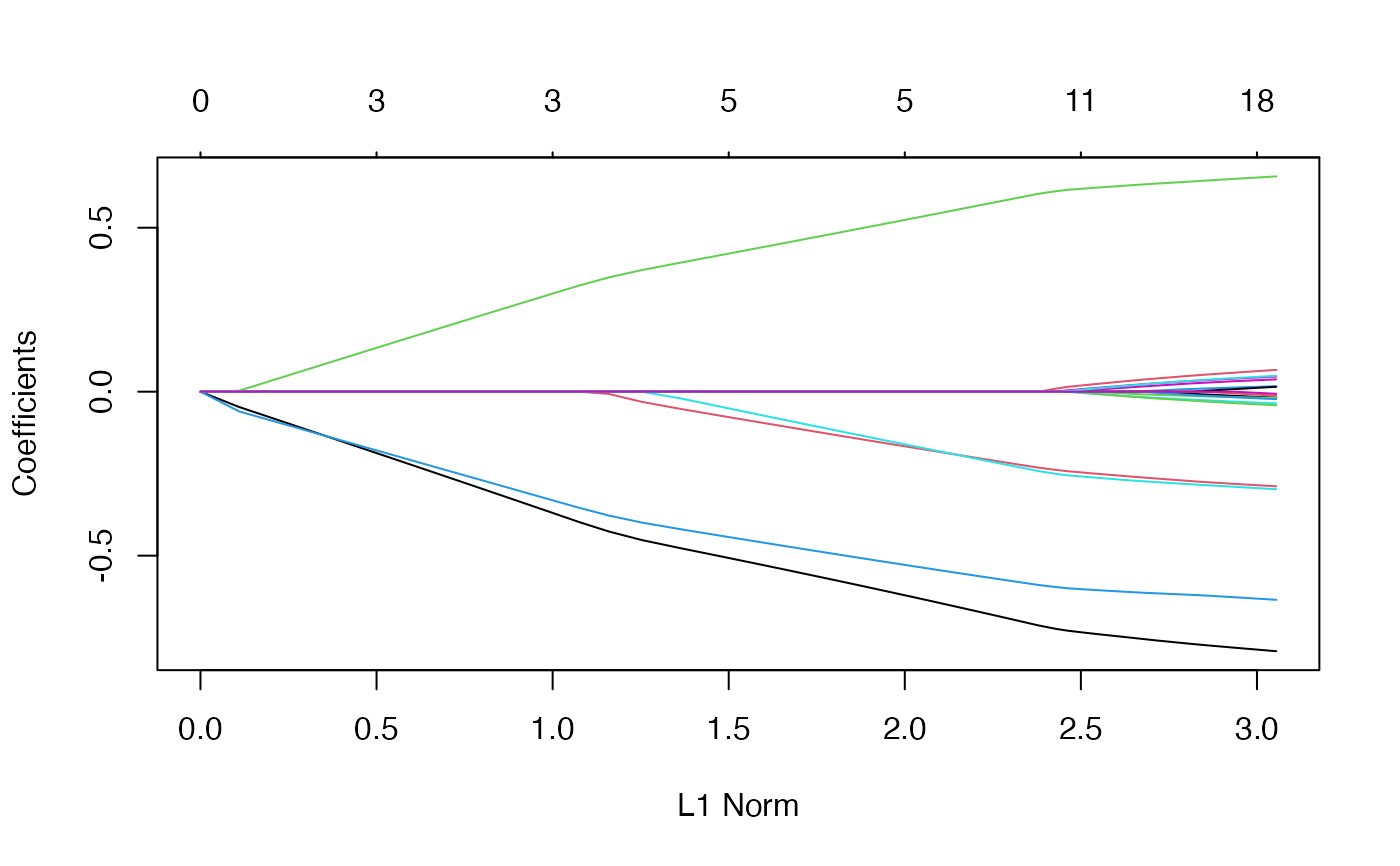pfit = predict(fit, x, s = 0.001, type = "response")
plot(pfit, y)


# Cox
set.seed(10101)
N = 1000
p = 30
nzc = p/3
x = matrix(rnorm(N * p), N, p)
beta = rnorm(nzc)
fx = x[, seq(nzc)] %*% beta/3
hx = exp(fx)
ty = rexp(N, hx)
tcens = rbinom(n = N, prob = 0.3, size = 1)  # censoring indicator
y = cbind(time = ty, status = 1 - tcens)  # y=Surv(ty,1-tcens) with library(survival)
fit = glmnet(x, y, family = "cox")
#> Warning: Starting in glmnet 5.1, the default Cox tie-handling method will change from 'breslow' to 'efron' (matching survival::coxph). To silence this message and lock in the v5.0 default, pass cox.ties = 'breslow' explicitly. To preview the v5.1 behavior, pass cox.ties = 'efron'.
plot(fit)


# Cox example with (start, stop] data
set.seed(2)
nobs <- 100; nvars <- 15
xvec <- rnorm(nobs * nvars)
xvec[sample.int(nobs * nvars, size = 0.4 * nobs * nvars)] <- 0
x <- matrix(xvec, nrow = nobs)
start_time <- runif(100, min = 0, max = 5)
stop_time <- start_time + runif(100, min = 0.1, max = 3)
status <- rbinom(n = nobs, prob = 0.3, size = 1)
jsurv_ss <- survival::Surv(start_time, stop_time, status)
fit <- glmnet(x, jsurv_ss, family = "cox")
#> Warning: Starting in glmnet 5.1, the default Cox tie-handling method will change from 'breslow' to 'efron' (matching survival::coxph). To silence this message and lock in the v5.0 default, pass cox.ties = 'breslow' explicitly. To preview the v5.1 behavior, pass cox.ties = 'efron'.

# Cox example with strata
jsurv_ss2 <- stratifySurv(jsurv_ss, rep(1:2, each = 50))
fit <- glmnet(x, jsurv_ss2, family = "cox")
#> Warning: Starting in glmnet 5.1, the default Cox tie-handling method will change from 'breslow' to 'efron' (matching survival::coxph). To silence this message and lock in the v5.0 default, pass cox.ties = 'breslow' explicitly. To preview the v5.1 behavior, pass cox.ties = 'efron'.

# Sparse
n = 10000
p = 200
nzc = trunc(p/10)
x = matrix(rnorm(n * p), n, p)
iz = sample(1:(n * p), size = n * p * 0.85, replace = FALSE)
x[iz] = 0
sx = Matrix(x, sparse = TRUE)
inherits(sx, "sparseMatrix")  #confirm that it is sparse
#> [1] TRUE
beta = rnorm(nzc)
fx = x[, seq(nzc)] %*% beta
eps = rnorm(n)
y = fx + eps
px = exp(fx)
px = px/(1 + px)
ly = rbinom(n = length(px), prob = px, size = 1)
system.time(fit1 <- glmnet(sx, y))
#>    user  system elapsed 
#>   2.227   0.002   2.229 
system.time(fit2n <- glmnet(x, y))
#>    user  system elapsed 
#>   1.955   0.003   1.960