assess performance of a 'glmnet' object using test data.

Given a test set, produce summary performance measures for the glmnet model(s)

assess.glmnet(
  object,
  newx = NULL,
  newy,
  weights = NULL,
  family = c("gaussian", "binomial", "poisson", "multinomial", "cox", "mgaussian"),
  ...
)

confusion.glmnet(
  object,
  newx = NULL,
  newy,
  family = c("binomial", "multinomial"),
  ...
)

roc.glmnet(object, newx = NULL, newy, ...)

Arguments

object: Fitted "glmnet" or "cv.glmnet", "relaxed" or "cv.relaxed" object, OR a matrix of predictions (for roc.glmnet or assess.glmnet). For roc.glmnet the model must be a 'binomial', and for confusion.glmnet must be either 'binomial' or 'multinomial'
newx: If predictions are to made, these are the 'x' values. Required for confusion.glmnet
newy: required argument for all functions; the new response values
weights: For observation weights for the test observations
family: The family of the model, in case predictions are passed in as 'object'
...: additional arguments to predict.glmnet when "object" is a "glmnet" fit, and predictions must be made to produce the statistics.

Value

assess.glmnet produces a list of vectors of measures. roc.glmnet a list of 'roc' two-column matrices, and confusion.glmnet a list of tables. If a single prediction is provided, or predictions are made from a CV object, the latter two drop the list status and produce a single matrix or table.

Details

assess.glmnet produces all the different performance measures provided by cv.glmnet for each of the families. A single vector, or a matrix of predictions can be provided, or fitted model objects or CV objects. In the case when the predictions are still to be made, the ... arguments allow, for example, 'offsets' and other prediction parameters such as values for 'gamma' for 'relaxed' fits. roc.glmnet produces for a single vector a two column matrix with columns TPR and FPR (true positive rate and false positive rate). This object can be plotted to produce an ROC curve. If more than one predictions are called for, then a list of such matrices is produced. confusion.glmnet produces a confusion matrix tabulating the classification results. Again, a single table or a list, with a print method.

Author

Trevor Hastie and Rob Tibshirani
Maintainer: Trevor Hastie hastie@stanford.edu

Examples


data(QuickStartExample)
x <- QuickStartExample$x; y <- QuickStartExample$y
set.seed(11)
train = sample(seq(length(y)),70,replace=FALSE)
fit1 = glmnet(x[train,], y[train])
assess.glmnet(fit1, newx = x[-train,], newy = y[-train])
#> $mse
#>         s0         s1         s2         s3         s4         s5         s6 
#> 10.5356884 10.0473027  9.5757375  8.7448060  8.0414304  7.4451552  6.8302096 
#>         s7         s8         s9        s10        s11        s12        s13 
#>  6.2099274  5.5979797  4.8918587  4.2620453  3.7367187  3.2983155  2.9322791 
#>        s14        s15        s16        s17        s18        s19        s20 
#>  2.6265064  2.3709330  2.1242795  1.9219451  1.7587268  1.6226452  1.5091624 
#>        s21        s22        s23        s24        s25        s26        s27 
#>  1.4144863  1.3354649  1.2694776  1.2143453  1.1682560  1.1297026  1.0974313 
#>        s28        s29        s30        s31        s32        s33        s34 
#>  1.0652936  1.0249928  0.9930414  0.9659219  0.9435578  0.9249772  0.9096485 
#>        s35        s36        s37        s38        s39        s40        s41 
#>  0.8970118  0.8866020  0.8773197  0.8703946  0.8648273  0.8609494  0.8597018 
#>        s42        s43        s44        s45        s46        s47        s48 
#>  0.8588511  0.8629691  0.8674411  0.8722799  0.8776263  0.8827885  0.8870380 
#>        s49        s50        s51        s52        s53        s54        s55 
#>  0.8911607  0.8951440  0.8989787  0.9030727  0.9070581  0.9109051  0.9145902 
#>        s56        s57        s58        s59        s60        s61        s62 
#>  0.9180974  0.9211897  0.9242868  0.9272307  0.9299921  0.9325693  0.9349674 
#>        s63        s64        s65        s66        s67        s68 
#>  0.9371937  0.9392563  0.9411642  0.9426805  0.9445011  0.9458195 
#> attr(,"measure")
#> [1] "Mean-Squared Error"
#> 
#> $mae
#>        s0        s1        s2        s3        s4        s5        s6        s7 
#> 2.6946299 2.6328780 2.5673994 2.4405206 2.3249133 2.2195763 2.1151049 2.0115127 
#>        s8        s9       s10       s11       s12       s13       s14       s15 
#> 1.9030069 1.7718821 1.6518698 1.5453805 1.4483515 1.3599423 1.2793871 1.2066589 
#>       s16       s17       s18       s19       s20       s21       s22       s23 
#> 1.1339882 1.0695296 1.0150683 0.9781225 0.9498621 0.9241123 0.9006501 0.8811996 
#>       s24       s25       s26       s27       s28       s29       s30       s31 
#> 0.8651666 0.8551227 0.8495833 0.8445360 0.8380969 0.8279767 0.8194392 0.8094367 
#>       s32       s33       s34       s35       s36       s37       s38       s39 
#> 0.7996659 0.7907266 0.7838971 0.7794754 0.7754465 0.7704058 0.7660117 0.7621631 
#>       s40       s41       s42       s43       s44       s45       s46       s47 
#> 0.7588402 0.7581804 0.7579210 0.7600092 0.7619297 0.7637101 0.7657734 0.7688329 
#>       s48       s49       s50       s51       s52       s53       s54       s55 
#> 0.7717302 0.7744494 0.7769264 0.7797273 0.7827940 0.7855762 0.7881095 0.7904177 
#>       s56       s57       s58       s59       s60       s61       s62       s63 
#> 0.7925209 0.7943038 0.7960365 0.7976354 0.7990963 0.8004283 0.8016421 0.8027481 
#>       s64       s65       s66       s67       s68 
#> 0.8037558 0.8046740 0.8053809 0.8062495 0.8068503 
#> attr(,"measure")
#> [1] "Mean Absolute Error"
#> 
preds = predict(fit1, newx = x[-train, ], s = c(1, 0.25))
assess.glmnet(preds, newy = y[-train], family = "gaussian")
#> $mse
#>       s1       s2 
#> 7.312414 1.498532 
#> attr(,"measure")
#> [1] "Mean-Squared Error"
#> 
#> $mae
#>        s1        s2 
#> 2.1976089 0.9470799 
#> attr(,"measure")
#> [1] "Mean Absolute Error"
#> 
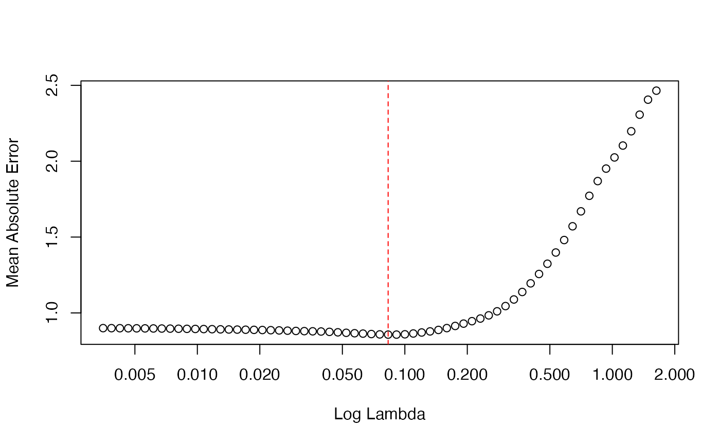
fit1c = cv.glmnet(x, y, keep = TRUE)
fit1a = assess.glmnet(fit1c$fit.preval, newy=y,family="gaussian")
plot(fit1c$lambda, log="x",fit1a$mae,xlab="Log Lambda",ylab="Mean Absolute Error")
abline(v=fit1c$lambda.min, lty=2, col="red")

data(BinomialExample)
x <- BinomialExample$x; y <- BinomialExample$y
fit2 = glmnet(x[train,], y[train], family = "binomial")
assess.glmnet(fit2,newx = x[-train,], newy=y[-train], s=0.1)
#> $deviance
#>       s1 
#> 1.037535 
#> attr(,"measure")
#> [1] "Binomial Deviance"
#> 
#> $class
#>        s1 
#> 0.1333333 
#> attr(,"measure")
#> [1] "Misclassification Error"
#> 
#> $auc
#> [1] 0.9351852
#> attr(,"measure")
#> [1] "AUC"
#> 
#> $mse
#>       s1 
#> 0.333371 
#> attr(,"measure")
#> [1] "Mean-Squared Error"
#> 
#> $mae
#>        s1 
#> 0.7909957 
#> attr(,"measure")
#> [1] "Mean Absolute Error"
#> 
plot(roc.glmnet(fit2, newx = x[-train,], newy=y[-train])[[10]])

fit2c = cv.glmnet(x, y, family = "binomial", keep=TRUE)
idmin = match(fit2c$lambda.min, fit2c$lambda)
plot(roc.glmnet(fit2c$fit.preval, newy = y)[[idmin]])

data(MultinomialExample)
x <- MultinomialExample$x; y <- MultinomialExample$y
set.seed(103)
train = sample(seq(length(y)),100,replace=FALSE)
fit3 = glmnet(x[train,], y[train], family = "multinomial")
confusion.glmnet(fit3, newx = x[-train, ], newy = y[-train], s = 0.01)
#>          True
#> Predicted   1   2   3 Total
#>     1      55  44  23   122
#>     2      29  82  17   128
#>     3      25  23 102   150
#>     Total 109 149 142   400
#> 
#>  Percent Correct:  0.5975 
fit3c = cv.glmnet(x, y, family = "multinomial", type.measure="class", keep=TRUE)
idmin = match(fit3c$lambda.min, fit3c$lambda)
confusion.glmnet(fit3c$fit.preval, newy = y, family="multinomial")[[idmin]]
#>          True
#> Predicted   1   2   3 Total
#>     1      71  22  13   106
#>     2      39 127  26   192
#>     3      32  25 145   202
#>     Total 142 174 184   500
#> 
#>  Percent Correct:  0.686