data(BinomialExample)
x <- BinomialExample$x
y <- BinomialExample$y

fit <- glmnet(x, y, family = "binomial")7 Binary classification
7.1 The logistic regression model
When the response variable is binary, the logistic regression model is often used. Let \(y\) denote the response variable, which can only take on values 0 or 1. The logistic regression model represents the class-conditional probabilities through a linear function of the predictors:
\[\begin{aligned} \text{Pr}(y=1 | \mathbf{x}) &= \dfrac{e^{(\beta_0 + \mathbf{x}^\top \beta)}}{1+e^{(\beta_0 + \mathbf{x}^\top \beta)}}, \\ \text{Pr}(y=0 | \mathbf{x}) &= \dfrac{1}{1+e^{(\beta_0 + \mathbf{x}^\top \beta)}} = 1 - \text{Pr}(y=1|\mathbf{x}), \end{aligned}\]
implying that the log-odds ratio is a linear function of the predictors:
\[\eta(\mathbf{x})=\log \dfrac{\text{Pr}(y=1 \mid \mathbf{x})}{\text{Pr}(y=0 \mid \mathbf{x})} = \beta_0 + \mathbf{x}^\top \beta. \tag{7.1}\]
If we let \(p(\mathbf{x}) = \text{Pr}(y=1 \mid \mathbf{x})\), we get the form of the logistic regression model commonly seen in textbooks:
\[y \sim \text{Bern}(p(\mathbf{x})), \qquad \text{logit}(p(\mathbf{x}))=\log \left( \frac{p(\mathbf{x})}{1-p(\mathbf{x})}\right) = \beta_0 + \mathbf{x}^\top \beta.\]
Here \(\text{Bern}(p)\) is the notation for a Bernoulli random variable with parameter \(p\), meaning that
\[y = \begin{cases} 1 &\text{with probability } p, \\ 0 &\text{with probability } 1-p. \end{cases}\]
We can fit this model by maximum likelihood estimation, or equivalently, by minimizing the negative log-likelihood (NLL). The log-likelihood for observation \(i\) is
\[\begin{aligned} \ell(y_i, p(\mathbf{x}_i)) &= y_i \log p(\mathbf{x}_i) + (1-y_i) \log (1-p(\mathbf{x}_i)) \\ &= y_i \log \left( \dfrac{e^{(\beta_0 + \mathbf{x}_i^\top \beta)}}{1+e^{(\beta_0 + \mathbf{x}_i^\top \beta)}} \right) + (1-y_i) \log \left( \dfrac{1}{1+e^{(\beta_0 + \mathbf{x}_i^\top \beta)}} \right) \\ &= y_i (\beta_0 + \mathbf{x}_i^\top \beta) - \log (1 + e^{(\beta_0 + \mathbf{x}_i^\top \beta)}). \end{aligned}\]
The logistic regression coefficient vector estimate is
\[(\hat\beta_0, \hat\beta) = \underset{(\beta_0, \beta) \in \mathbb{R}^{p+1}}{\text{argmin}} \; -\sum_{i=1}^n \ell (y_i, \beta_0 + \mathbf{x}_i^\top \beta).\]
We can fit the logistic regression model in R with the glm function from the stats package, specifying the option family = binomial.
7.2 Regularized logistic regression
Logistic regression is plagued with degeneracies when \(p > N\) and exhibits wild behavior even when \(p\) is close to \(N\). The elastic net penalty alleviates these issues, and regularizes and selects variables as well.
To extend the regularized linear regression models — ridge, lasso, and elastic net — to the binary response setting, we modify the objective function that they aim to minimize. In Chapter 2, we defined the regularized regression solutions as the coefficient vector that minimizes a combination of the residual sum of squares (RSS) and a penalty on the size of the coefficients. Similarly, in the binary response setting, we define the regularized solutions as the coefficient vector that minimizes a combination of the NLL and the elastic net penalty:
\[(\hat\beta_0, \hat\beta) = \underset{(\beta_0, \beta) \in \mathbb{R}^{p+1}}{\text{argmin}} \; -\frac{1}{n} \sum_{i=1}^n \ell (y_i, \beta_0 + \mathbf{x}_i^\top \beta) + \lambda \left(\frac{1-\alpha}{2}\|\beta \|_2^2 + \alpha \|\beta \|_1 \right). \tag{7.2}\]
As before, setting \(\alpha = 0\) gives the ridge solution (shrinkage) and \(\alpha = 1\) gives the lasso solution (sparsity); values between 0 and 1 yield a blend of the two approaches.
To fit a regularized logistic regression model with the glmnet package, you just have to include the family = "binomial" argument in the glmnet call. Here is an example:
Recall that by default, glmnet fits a lasso model (\(\alpha = 1\)). As with family = "gaussian", the returned fit object comes equipped with plot, print, coef and predict methods. They work in very much the same way for family = "binomial": we just highlight the differences below.
7.2.1 The predict method
For family = "gaussian", the predict method returned the predictions for the fitted model, i.e. \(\hat{y} = \hat{\beta}_0 + \mathbf{x}^\top \hat\beta\). For family = "binomial", there are 3 possible options, depending on the type argument passed to predict:
type = "link"(default) returns the linear predictors \(\hat{\eta} = \hat{\beta}_0 + \mathbf{x}^\top \hat\beta\).type = "response"returns the fitted probabilities \(\hat{p} = \dfrac{\exp (\hat{\beta}_0 + \mathbf{x}^\top \hat\beta)}{1 + \exp (\hat{\beta}_0 + \mathbf{x}^\top \hat\beta)}\).type = "class"returns the class label corresponding to the maximum fitted probability.
Here is an example of the return value for predict with type = "class":
predict(fit, newx = x[1:5,], type = "class", s = 0.01)
#>      s=0.01
#> [1,] "0"
#> [2,] "1"
#> [3,] "1"
#> [4,] "0"
#> [5,] "1"
7.2.2 Using different error measures for cross-validation
You can run cross-validation (CV) for the \(\lambda\) hyperparameter for a regularized logistic regression model by calling cv.glmnet with family = "binomial". Logistic regression has several model performance measures: you can specify which performance measure cv.glmnet should compute using the type.measure argument. Here are the possibilities:
type.measure = "deviance"(default): deviancetype.measure = "mse": Brier score (squared loss)type.measure = "mae": mean absolute errortype.measure = "class": misclassification errortype.measure = "auc": area under the receiver operating characteristic (ROC) curve
You can see what measures are available for any family by executing glmnet.measures().
The lambda.1se and lambda.min values are computed based on the type.measure argument used. Here is an example of using misclassification error for CV:
set.seed(1)
cvfit <- cv.glmnet(x, y, family = "binomial", type.measure = "class")
plot(cvfit)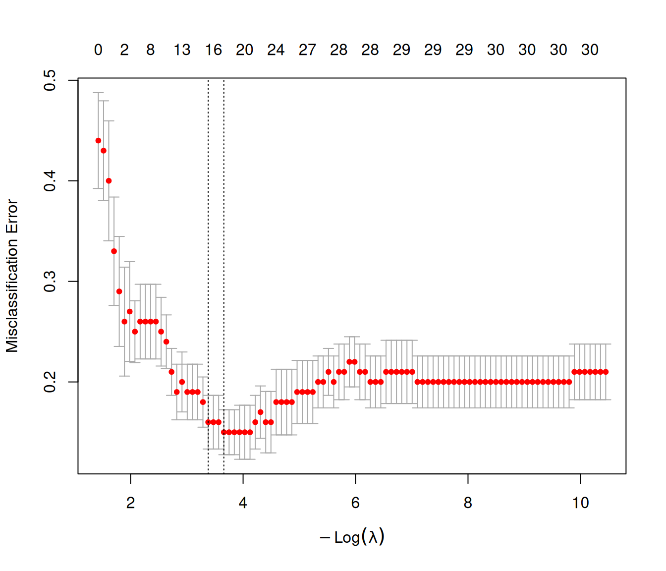
7.2.3 When should I use each error measure?
Here, we define \(\hat p_i = \dfrac{e^{(\hat\beta_0 + \mathbf{x}_i ^\top \hat\beta)}}{1+e^{(\hat\beta_0 + \mathbf{x}_i ^\top \hat\beta)}}\) as the predicted probability from our model for observation \(\mathbf{x}_i\), and \(\hat{y}_i = I(\hat{p}_i \geq 0.5)\) as the predicted class.
Deviance (
type.measure = "deviance")Formula: \(-\displaystyle\frac{2}{n} \sum_{i=1}^n \left( y_i \log(\hat{p}_i) + (1 - y_i) \log(1 - \hat{p}_i) \right)\)
Good for:
A measure like RSS for likelihood-based inference.
Deviance is a proper scoring rule (see Section 7.4.1).
Avoid if: You only care about classification (and not probability estimates).
Brier score (
type.measure = "mse")Formula: \(\displaystyle\frac{1}{n} \sum_{i=1}^n (y_i - \hat{p}_i)^2\)
Good for:
Probability calibration.
Brier score is a proper scoring rule.
Avoid if: You have imbalanced classes. In this case, the Brier score can be misleadingly small, and favor models that reflect class priors rather than model discrimination.
Mean absolute error (
type.measure = "mae")Formula: \(\displaystyle\frac{1}{n} \sum_{i=1}^n |y_i - \hat{p}_i|\)
Good for: Probability accuracy.
Avoid if: You need a proper scoring rule (the Brier score would be preferred).
Misclassification error (
type.measure = "class")Formula: \(\displaystyle\frac{1}{n} \sum_{i=1}^n \mathbb{1} (y_i \neq \hat{y_i})\)
Best for:
Classification accuracy.
Datasets where false positives and false negatives have equal importance.
Avoid if:
You care about probability prediction or ranking predictions.
You have imbalanced classes.
You need a proper scoring rule.
Area under the ROC curve (
type.measure = "auc")Formula:
Sort observations by \(\hat{p}_i\) in descending order.
Compute the True Positive Rate (TPR) and False Positive Rate (FPR) at all possible classification thresholds.
Compute the AUC using the trapezoidal rule: \(\displaystyle\sum_{i=1}^{n-1} (\text{FPR}_{i+1} - \text{FPR}_i) \times \frac{\text{TPR}_{i+1} + \text{TPR}_i}{2}\)
Best for: Imbalanced datasets, since AUC evaluates discrimination.
Avoid if:
Probability calibration is important.
You need a proper scoring rule.
You primarily care about class assignments rather than probabilities
NoteThe AUC reported by
cv.glmnetis the average AUC across folds, not the AUC computed from the entire dataset. These two quantities may differ significantly. See Appendix C for more details.
The AUC measures to what extent the order of the fitted probabilities lines up with the order of the 0/1 binary class labels. It is the fraction of times that the predicted probability for a randomly selected “1” observation exceeds the predicted probability for a randomly selected “0” observation. So an AUC of 1 means perfect ordering, and an AUC of 0.5 means random guessing.
7.3 Working with imbalanced classes
It is common that the class we are trying to predict is observed much less frequently than the other. For example, fraud is rare in financial data and click-throughs are uncommon in online advertising, often with just 0.01% to 1% of the data being in the minority class. Here, we share strategies for model-fitting in this setting.
7.3.1 Case-control sampling, or downsampling the majority class
In case-control sampling, we typically keep all observations from the minority class (cases), and we undersample the majority class (controls). This is common in retrospective studies in medicine. For example, suppose we wish to train a model to predict heart attack using data from a hospital. Relative to the entire hospital population, heart attacks are rare. In this case, a sensible thing to do would be to collect data from every person who did have a heart attack, and then take a sample of patients who did not have a heart attack (instead of using all patients who did not have a heart attack).
Something similar happens when datasets are very large. For example, in advertising, website traffic may be very high, while the click-through rate of a particular ad may be very low (as few as one click every 10,000 visits). In this case, we could choose to downsample the majority class to a more manageable ratio (e.g., 10:1), which improves training efficiency.
When we downsample the majority class, we can still estimate the coefficients for each feature accurately. However, the intercept will not reflect true prevalence of heart attack in the population because the class proportions in the training data were altered. To produce well-calibrated probabilities, we can correct the intercept \(\hat{\beta}_0\) after model fitting, using the adjustment:
\[\tilde{\beta}_0 = \hat{\beta}_0 + \log\left(\frac{\pi}{1 - \pi}\right) - \log\left(\frac{\tilde{\pi}}{1 - \tilde{\pi}}\right), \tag{7.3}\]
where \(\pi\) is the true fraction of positive cases in the population and \(\tilde{\pi}\) is the fraction of positive cases in the downsampled data.
So, how much should we downsample? The answer to this depends on the problem, computing resources and data, but a rule of thumb is to retain 5–10 majority-class samples for each minority-class sample. While more data generally reduces variance in coefficient estimates, the improvement in variance begins to taper off after about 5–6 majority samples per minority sample. For more about this (and case-control sampling), see Hastie and Tibshirani (2022).
7.3.2 Reweighting the data
Another strategy for handling class imbalance is to assign weights to each observation during model fitting. The idea is simple: upweight examples from the minority class to increase their influence during model training. This is mainly useful in cross-validation, and allows us to give more focus to the minority class when picking say \(\lambda\). Importantly, using weights mean that no data is thrown away – unlike downsampling described above.
Suppose only 1% of your data belongs to the positive class. You might assign a weight of 1 to each negative observation and a weight of 99 to each minority-class (positive) observation so that the total weight for each class will be equal.
Assigning weights in glmnet and cv.glmnet is straightforward using the weights argument:
wt.class1 <- 1 / sum(y == 1)
wt.class0 <- 1 / sum(y == 0)

weights <- ifelse(y == 1, wt.class1, wt.class0)

cvfit <- glmnet(x, y,
                family = "binomial",
                weights = weights)
Note that glmnet normalizes the weights internally so they sum to the number of observations in the dataset.
As with downsampling, weighting distorts the marginal class probabilities. If your goal is to make probability predictions, you may still need to correct the intercept as in Equation 7.3.
7.4 Additional notes
7.4.1 What is a scoring rule?
A scoring rule is a function that assigns a score to a probabilistic model based on how well the model predictions match the observed outcomes. Scoring rules are often used to perform model selection: we typically prefer models with better scores.
In practice, a scoring rule \(S(\hat{p}, y)\) is a function of predicted probabilities \(\hat{p}\) and the observed response \(y\). If, however, we knew the true probability distribution \(p\), then we could compute the score \(S(\hat{p}, p)\) to compare our predictions to the true probabilities.
A scoring rule is proper when \(S(p, p) \geq S(\hat{p}, p)\) for all \(\hat{p}\). This means that the scoring rule is maximized for models that predict the true distribution. To maximize a proper scoring rule, a model must give “honest” predictions – e.g. it should not be overconfident and predict \(0.9\) when the true probability is \(0.7\).
A strictly proper scoring rule satisfies \(S(p, p) > S(\hat{p}, p)\).
Misclassification error is an example of an improper scoring rule: it ignores predicted probabilities and instead uses hard classification assignments. For example, if the threshold for classification is \(0.5\), a prediction of \(0.9\) is treated the same as a prediction of \(0.7\). This does not mean that misclassification error is bad - it simply helps us understand that it may not always be sufficient to distinguish between models.
Note: There are, however, other issues with misclassification error that are worth considering! Harrell (2017) shows examples of misclassification error being optimized by choosing the wrong predictive features and giving them the wrong weights.
7.4.2 More information
For algorithmic details on how we solve Equation 7.2 efficiently, see Friedman et al. (2010).
For more about error measures, see Harrell (2017) and Tay (2019).