22 glmnet in python: the adelie package

Python (the programming language) is quickly becoming the de factor standard programming language for machine learning (ML) and artificial intelligence (AI) in industry. Its popularity is driven by a combination of code readability, an active open-source ecosystem, and easy integration with production systems.

While R remains an important programming language in specific domains (e.g. statistics, epidemiology, public health), it is increasingly important for statisticians and data scientists to be conversant in Python as well.

Thus far, we have presented glmnet’s routines for fitting various elastic net models in R. In this chapter, we demonstrate how one can fit such models in Python via the adelie package.

22.1 The adelie package

adelie is a high-performance package for solving lasso, elastic net, group lasso, and group elastic net problems. Here are the key advantages and benefits of the package:

adelie supports a variety of matrix classes optimized for large-scale data with specialized structures.
adelie can fit many different types of generalized linear models (GLMs) for different data types.
adelie is easily extensible: users can extend adelie’s matrix and GLM classes for greater customization.
Many core operations in adelie, including matrix-vector multiplications and the computation of gradients, Hessians, and losses for GLMs, have been extensively optimized and parallelized.

adelie is available as both a Python package and an R package. We focus on the Python package in this chapter. (We describe how to use adelie in R as well as other types of models that adelie can fit in Chapter 25).

22.2 adelie in python: a crash course

In this section, we show the basic workflow for using the adelie python package to run the elastic net with cross-validation (CV). (See the official user guide for more documentation and examples of adelie.)

First, let’s load the packages we’ll need for this walkthrough. The adelie python package is available through the pip package manager; see this for other installation options.

import adelie as ad
import numpy as np
import matplotlib.pyplot as plt

Next, let’s generate some simulated data:

n = 100      # number of training observations
n_test = 10  # number of test observations
p = 1000    # number of features

np.random.seed(0)
# adelie works fastest with column-major (Fortran-ordered) matrices, and warns
# if given a row-major (C-ordered) one, which is numpy's default.
X = np.asfortranarray(np.random.normal(0, 1, (n, p)))
y = X[:, -1] * np.random.normal(0, 1) + np.random.normal(0, 1, n)

X_test = np.asfortranarray(np.random.normal(0, 1, (n_test, p)))
y_test = X_test[:, -1] * np.random.normal(0, 1) + np.random.normal(0, 1, n_test)

We can use the cv_grpnet function to fit the elastic net¹ with CV: the code below does so for the Gaussian GLM (i.e. family = "gaussian" in the glmnet function). The X argument takes in the input matrix, while the response variable is passed via the glm argument. (As with glmnet, the \(\alpha\) parameter can be set via the alpha argument, and its default value is 1 which corresponds to the lasso.)

np.random.seed(42)
cvstate = ad.cv_grpnet(
    X=X,
    glm=ad.glm.gaussian(y=y),
)

  0%|          | 0/100 [00:00:00<?, ?it/s]

100%|██████████| 100/100 [00:00:00<00:00:00, 15495.25it/s] [dev:94.9%]

100%|██████████| 100/100 [00:00:00<00:00:00, 13894.19it/s] [dev:94.9%]



  0%|          | 0/109 [00:00:00<?, ?it/s]

100%|██████████| 109/109 [00:00:00<00:00:00, 12726.24it/s] [dev:96.1%]

100%|██████████| 109/109 [00:00:00<00:00:00, 12261.35it/s] [dev:96.1%]



  0%|          | 0/103 [00:00:00<?, ?it/s]

100%|██████████| 103/103 [00:00:00<00:00:00, 11439.17it/s] [dev:94.6%]

100%|██████████| 103/103 [00:00:00<00:00:00, 10257.65it/s] [dev:94.6%]



  0%|          | 0/102 [00:00:00<?, ?it/s]

100%|██████████| 102/102 [00:00:00<00:00:00, 12381.42it/s] [dev:95.9%]

100%|██████████| 102/102 [00:00:00<00:00:00, 10845.29it/s] [dev:95.9%]



  0%|          | 0/100 [00:00:00<?, ?it/s]

100%|██████████| 100/100 [00:00:00<00:00:00, 12564.74it/s] [dev:95.2%]

100%|██████████| 100/100 [00:00:00<00:00:00, 10750.26it/s] [dev:95.2%]

You can modify the glm argument to run the elastic net with CV for other GLM families. For example, glm=ad.glm.binomial(y=y) will run logistic regression, while glm=ad.glm.poisson(y=y) will run Poisson regression. The adelie package has implemented a number of these families in the adelie.glm module, details on each family can be found in the API reference. It is also possible to create your own family to be used by cv_grpnet: see this reference for details.

The cv_grpnet function returns a class CVGrpnetResult object. It comes equipped with a plot_loss method that plots the CV error against lambda:

cvstate.plot_loss()

(<Figure size 864x576 with 1 Axes>,
 <Axes: title={'center': 'K-Fold CV Mean Loss'}, xlabel='$-\\log(\\lambda)$', ylabel='Mean Loss'>)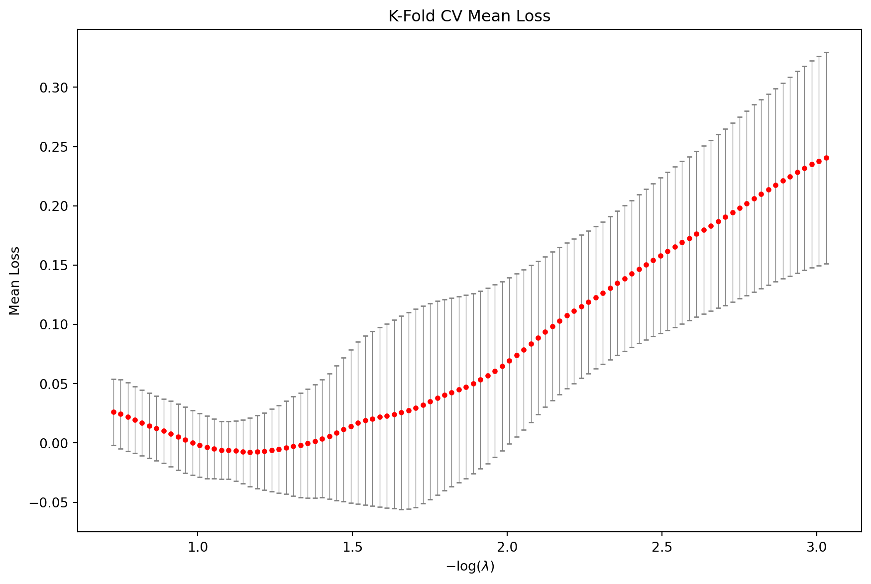

The lambda.min value (i.e. the lambda corresponding to the best CV error) can be extracted as such:

# index of lambda.min within the lambda sequence
print(cvstate.best_idx)

# lambda.min value
print(cvstate.lmdas[cvstate.best_idx])

19
0.3106533704812743

At the time of writing, to get coefficients and predictions at the lambda.min value requires a bit more work. First, we refit the elastic net on the lambda path up to the best lambda² using grpnet (this fits the group elastic net without CV):

state = ad.grpnet(
    X=X,
    glm=ad.glm.gaussian(y=y),
    lmda_path = cvstate.lmdas[:(cvstate.best_idx+1)],
)

  0%|          | 0/20 [00:00:00<?, ?it/s]

100%|██████████| 20/20 [00:00:00<00:00:00, 15493.50it/s] [dev:13.3%]

100%|██████████| 20/20 [00:00:00<00:00:00, 12616.89it/s] [dev:13.3%]

This returns a state object which represents the state of the optimizer. The model coefficients at the lambda.min value can be pulled out in the following manner:

print(state.betas[cvstate.best_idx,:])
print(state.intercepts[cvstate.best_idx])

<Compressed Sparse Row sparse matrix of dtype 'float64'
    with 4 stored elements and shape (1, 1000)>
  Coords    Values
  (0, 99)   0.021327770055327624
  (0, 916)  0.03415305353779968
  (0, 989)  -0.0032104769692209855
  (0, 999)  -0.1627236610111638
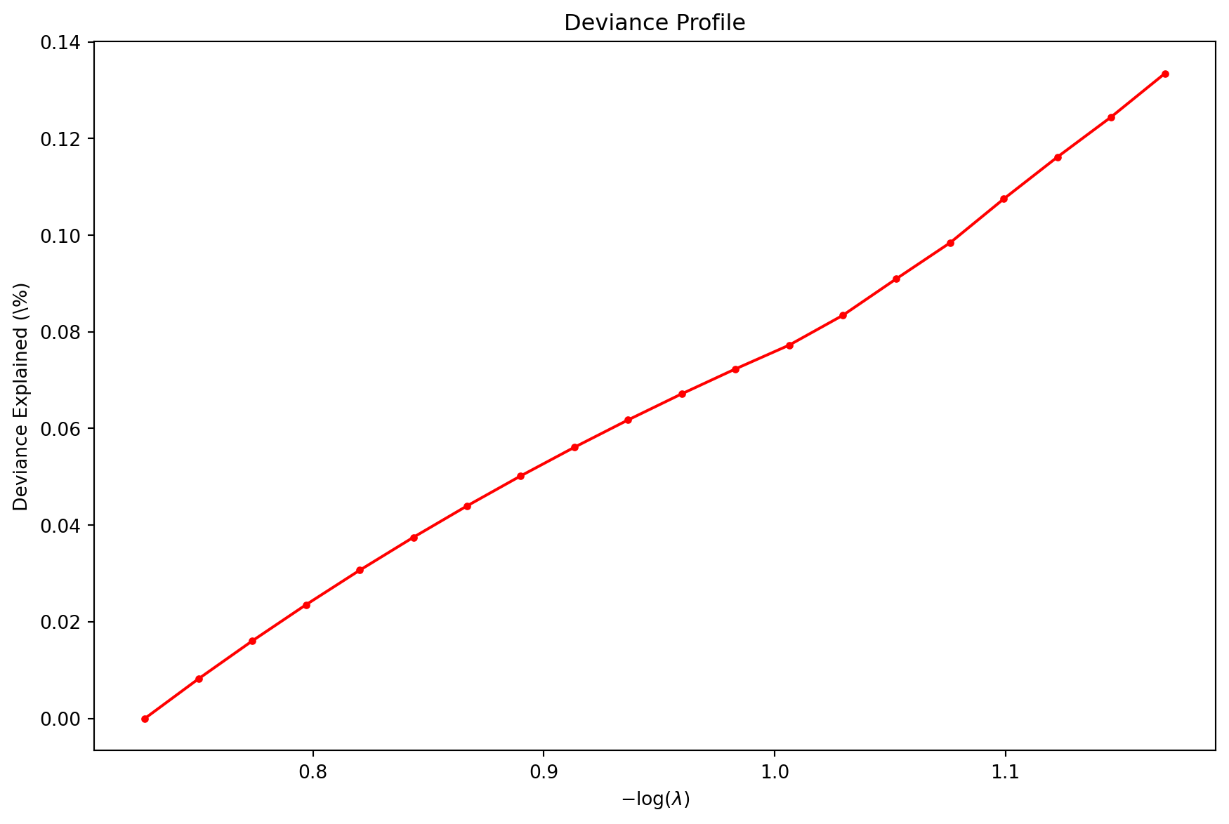
0.029908784411029274

The code below shows how you can make coefficient and deviance plots:

dg = ad.diagnostic.diagnostic(state=state)
dg.plot_coefficients()
dg.plot_devs()

(<Figure size 864x576 with 1 Axes>,
 <Axes: title={'center': 'Deviance Profile'}, xlabel='$-\\log(\\lambda)$', ylabel='Deviance Explained (\\%)'>)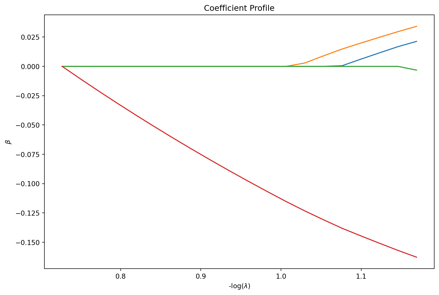

The linear predictions \(\hat{y}= \hat{\beta}_0 + \hat{\beta}^\top x\) for the training data can be accessed directly with dg.linear_preds:

# 20 lambda values x 100 observations
print(dg.linear_preds.shape)

(20, 100)

The code below can be used to obtain predictions at every lambda value the model was fit to:

etas = ad.diagnostic.predict(
  X=X_test,
  betas=state.betas,
  intercepts=state.intercepts,
)

# 20 lambda values x 10 test observations
print(etas.shape)

(20, 10)

The code can be modified to return just the linear predictions at the lambda.min value (by construction, this corresponds to the last lambda value we used in fitting the model a second time):

etas_lambda_min = ad.diagnostic.predict(
  X=X_test,
  betas=state.betas[-1,],
  intercepts=state.intercepts[-1],
)

print(etas_lambda_min)

[[-0.10301036  0.21540329 -0.03702336  0.09169884  0.0677207   0.12977019
   0.05845629  0.04366172 -0.21764467  0.1928459 ]]

22.3 A comparison with scikit-learn

scikit-learn (also known as sklearn) an open-source Python library for a vast array of machine learning tools. As one might expect, scikit-learn has its own implementation of the elastic net. The implementation names the elastic net hyperparameters differently from glmnet and adelie: alpha in glmnet and adelie corresponds to l1_ratio in scikit-learn, and somewhat confusingly lambda in glmnet and adelie corresponds to alpha in scikit-learn. Since we are focused on scikit-learn in this section, we will follow their terminology here. There are three functions relevant to fitting the elastic net:

sklearn.linear_model.ElasticNet fits an elastic net model for a single (alpha, l1_ratio) setting.
sklearn.linear_model.enet_path fits a series of elastic net models for a single l1_ratio value and a path of alpha values (just like glmnet::glmnet and ad.grpnet).
sklearn.linear_model.ElasticNetCV fits the elastic net model with CV. It can do CV for both alpha and l1_ratio at the same time. If l1_ratio consists of just one value, this corresponds to the functionality provided by glmnet::cv.glmnet and ad.cv_grpnet.

As data analysis pipelines sometimes assume scikit-learn API for the models, you have the option of using adelie with scikit-learn-style API to allow for seamless integration. For example, this vignette demonstrates how to run \(k\)-fold cross-validation and get predictions at the lambda.min value with this API. We note, however, that this scikit-learn-style solver is a simple wrapper of the more generic tools provided in adelie, and so is less flexible (e.g. you cannot give it a user-specified GLM family, no diagnostic plots).

See Appendix D for code illustrating how to match the output from the two elastic net implementations.

The cv_grpnet function actually fits the group elastic net. However, when each input feature is its own group (the default setting for cv_grpnet), the group elastic net simplifies to the elastic net model which glmnet fits. We talk more about groups and the group elastic net in Chapter 25.↩︎
Since warm start is crucial for coordinate descent to work well, we recommend fitting with a path of lambda values even if you are only interested in the model at a single lambda value.↩︎