18  Filtering

The glmnet and cv.glmnet functions have an exclude argument which accepts a vector of indices, indicating which variables should be excluded from the fit, i.e., get zeros for their coefficients.

18.1 Excluding variables dynamically

More intriguingly, the exclude argument can also accept a function as input. The idea is that variables can be filtered based on some property before any models are fit. One use case for this is in genomics, where we often want to exclude features which are too sparse, being non-zero for the vast majority of observations.

The code examples below shows the two different ways of using the exclude argument. In this example, we want to exclude all variables that are more than 80% sparse. Here is the filter function describing this:

filter <- function(x, ...) which(colMeans(x == 0) > 0.8)

The function takes in the x matrix and returns a vector of column indices which should be dropped before fitting the model.

For the first way of using the exclude argument, we manually determine which column indices should be removed before fitting the model and explicitly pass that index list to glmnet:

data("QuickStartExample")
x <- QuickStartExample$x
y <- QuickStartExample$y

# randomly set entries in the X matrix to zero
set.seed(1)
x[sample(seq(length(x)), 1600)] <- 0

# feature indices to be excluded from model fitting
exclude <- filter(x)
exclude
#>  [1]  1  2  3  4  5  7  8 12 14 15 17 18

fit1 <- glmnet(x, y, exclude = exclude)

For the second way of using the exclude argument, we pass the filter function directly to the exclude argument. The two methods return the same result except for the function call that produced the fit.

fit2 <- glmnet(x, y, exclude = filter)
all.equal(fit1, fit2)
#> [1] "Component \"call\": target, current do not match when deparsed"

18.2 Filtering for cross-validation

It is easy to make mistakes when performing cross-validation (CV) with data-dependent filter functions (or more generally, any data-dependent pre-processing). The following \(K\)-fold CV workflow is commonly used but gives biased CV error estimates:

1. Use the entire training dataset \(D\) to determine which input features should be dropped. Let \(f(D)\) denote the dataset after these features are dropped.
2. For \(k = 1, \dots, K\):
   1. Fit the model on \((f(D))_{-k}\) (rows of \(f(D)\) not in fold \(k\)).
   2. Evaluate CV error on \((f(D))_k\) (rows of \(f(D)\) in fold \(k\)).

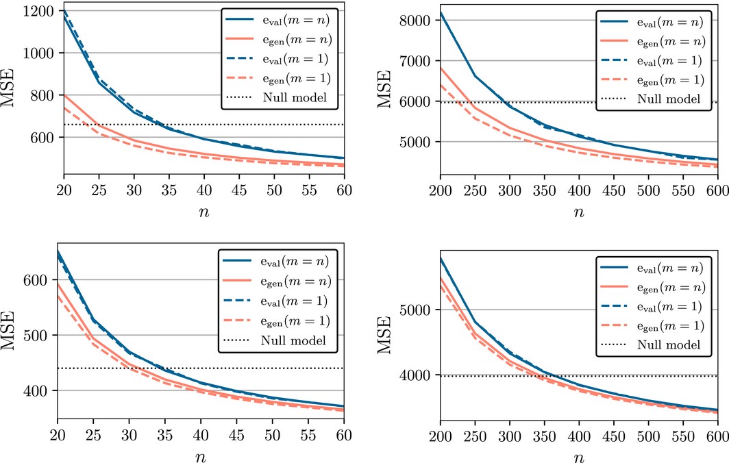
It is commonly known that using the response variable \(y\) in Step 1 above induces bias in the CV error estimates. It is less commonly known that such bias can exist even if pre-processing in Step 1 is unsupervised, i.e. not using \(y\) at all!

The figure below, taken from Moscovich and Rosset (2022), demonstrates how large the bias of the workflow above could be in the context of filtering variables based on variance in high-dimensional linear regression¹. \(n\) represents the number of observations, \(e_{val}\) (blue lines) represents the CV error estimate and \(e_{gen}\) (orange lines) represents the true value that CV is trying to estimate. \(m = n\) corresponds to two-fold CV while \(m = 1\) corresponds to leave-one-out CV. In the 4 settings presented in this figure, there is a gap between the estimates and the true value, with the gap being larger when the number of observations is smaller.

This is the correct \(K\)-fold CV workflow for estimating CV error when data-dependent filtering is involved:

1. For \(k = 1, \dots, K\):
   1. Use \(D_{-k}\) (rows of \(D\) not in fold \(k\)) to determine which input features should be dropped. Let \(f_k(D_{-k})\) denote the dataset after these features are dropped.
   2. Fit the model on \(f_k(D_{-k})\).
   3. Evaluate CV error on \(f_k(D_k)\) (rows in fold \(k\), but only the features we keep for this value of \(k\)).

A key difference between this correct workflow and the incorrect one is in this workflow, the input features which are dropped can vary from fold to fold.

Assigning a function to the exclude argument allows us to perform CV correctly, as in the workflow above. If a filtering function is given as the exclude argument, cv.glmnet will apply that function separately to each training fold, hence accounting for any bias that may be incurred by the variable filtering. (This is not possible when assigning a vector of indices to exclude: in that case, the excluded variables are forced to be the same across folds.)

18.3 General form for the filter function

The most general form of the filter function is

filter <- function(x, y, weights, ...) {}

Yes: you are allowed to use the response y and observation weights weights in the filtering criterion if it makes sense². As in the example of excluding sparse variables, these two arguments can be omitted, but the ... must always be there.

18.4 Parameterizing the filter function

Note that any other arguments in a user’s filter function are ignored. If we want to add parameters to our filtering function, how can we do so? The safest way to achieve this is to write a filter generator function, that produces a filter function as its output.

Build on the feature sparsity example, let’s say we want to exclude variables above a user-specified level of sparsity, not just 80%. Here is the filter generator function:

sparsity <- function(fraction = 0.7) {
  function(x, ...) which(colMeans(x == 0) > fraction)
}

If we want to exclude variables whose proportion of zero values exceeds fraction, we simply add exclude = sparsity(fraction) to the glmnet call. The example below demonstrates the correctness of this approach (the fits only differ in the function call):

filter <- function(x, ...) which(colMeans(x == 0) > 0.8)
fit1 <- glmnet(x, y, exclude = filter)
fit2 <- glmnet(x, y, exclude = sparsity(0.8))
all.equal(fit1, fit2)
#> [1] "Component \"call\": target, current do not match when deparsed"

Running glmnet again but now only excluding variables that are more than 85% sparse is easy:

fit <- glmnet(x, y, exclude = sparsity(0.85))

More importantly, we can now do cross-validation the correct way as well:

cvfit <- cv.glmnet(x, y, exclude = sparsity(0.85))

The filter function is applied separately on each training fold.

18.5 Filter function examples

We end this chapter with two examples of commonly used filters.

18.5.1 Removing features with the lowest variance

In genomics where the x matrix can be very wide, we often filter features based on variance. Let’s use gene expression arrays as an example. All else being equal, if a particular gene’s expression does not vary much in our training data, then it is unlikely that it is strongly predictive of the response. We might want to exclude genes with expression variance below some threshold.

As a first step, we write a function that efficiently computes the column-wise variance for a wide matrix:

uvar <- function(x, means = FALSE) {
  # if means = TRUE, the column means and variances are returned, 
  # otherwise just the variances
  m <- colMeans(x)
  n <- nrow(x)
  x <- x - outer(rep(1, n), m)
  v <- colSums(x^2) / (n - 1)
  if (means) list(mean = m, var = v) else v
}

Next, we write a filter generator function that takes a parameter q and returns a filter function that gives the fraction q of variables with the lowest variance:

vfilter <- function(q = 0.3) {
  function(x, ...) {
    v <- uvar(x)
    which(v < quantile(v, q))
  }
}

If we want to exclude the bottom 40% of genes in terms of variance before model-fitting, and run CV properly to select the tuning parameters, we would do the following:

cvfit <- cv.glmnet(x, y, exclude = vfilter(0.4))

18.5.2 Removing features based on \(t\)-statistic

In this example, our response y is binary. Split the training data observations into two groups based on the value of y. If an input variable is strongly predictive of y, we would expect the value of the two-sample \(t\)-statistic for this variable to be significant (i.e. large absolute value). We want to exclude variables with low values of this statistic.

First, we write an efficient function for computing the \(t\)-statistics for each input feature. (The function uvar is taken from Section 18.5.1.) We include an offset s0 for the denominator of the \(t\)-statistic: we can set it to a small positive number if we want to avoid issues associating with dividing by zero.

ut.test <- function(x, y, s0 = 0) {
  ni <- table(y); n <- sum(ni)
  if(length(ni) != 2) stop("Only two-sample t-test here")
  index <- seq(n)
  mv <- tapply(index, y, function(i, x) uvar(x[i, ], means = TRUE), x = x)
  ss <- ((ni[1] - 1) * mv[[1]]$var  + (ni[2] - 1) * mv[[2]]$var)
  sd <- sqrt(ss * (1 / ni[[1]] + 1 / ni[[2]]) / (n - 2))
  numer <- mv[[1]]$mean - mv[[2]]$mean
  numer / (sd + s0)
}

Next, we write a filter generator function that takes a parameter q and returns a filter function that gives the fraction q of input features with the smallest \(t\)-statistics by absolute value:

tfilter <- function(q = 0.3, s0 = 0) {
  function(x, y, ...) {
    abs_tstats <- abs(ut.test(x, y, s0 = s0))
    which(abs_tstats < quantile(abs_tstats, q))
  }
}

If we want to exclude the bottom 20% of genes in terms of variance before model-fitting, and select the model via CV, we would do the following:

cvfit <- cv.glmnet(x, y, exclude = tfilter(0.2))

Moscovich, Amit, and Saharon Rosset. 2022. “On the Cross-Validation Bias Due to Unsupervised Preprocessing.” Journal of the Royal Statistical Society Series B: Statistical Methodology 84 (4): 1474–502. https://doi.org/10.1111/rssb.12537.

Paul, Debashis, Eric Bair, Trevor Hastie, and Robert Tibshirani. 2008. ““Preconditioning” for Feature Selection and Regression in High-Dimensional Problems.” The Annals of Statistics 36 (4). https://doi.org/10.1214/009053607000000578.

---

1. The paper contains full details of the simulation, as well as theoretical reasons for this bias. Code for reproducing this figure can be found here.

2. One example of this is preconditioning (Paul et al. 2008).