library(MASS)
data(Boston)
str(Boston)
#> 'data.frame':    506 obs. of  14 variables:
#>  $ crim   : num  0.00632 0.02731 0.02729 0.03237 0.06905 ...
#>  $ zn     : num  18 0 0 0 0 0 12.5 12.5 12.5 12.5 ...
#>  $ indus  : num  2.31 7.07 7.07 2.18 2.18 2.18 7.87 7.87 7.87 7.87 ...
#>  $ chas   : int  0 0 0 0 0 0 0 0 0 0 ...
#>  $ nox    : num  0.538 0.469 0.469 0.458 0.458 0.458 0.524 0.524 0.524 0.524 ...
#>  $ rm     : num  6.58 6.42 7.18 7 7.15 ...
#>  $ age    : num  65.2 78.9 61.1 45.8 54.2 58.7 66.6 96.1 100 85.9 ...
#>  $ dis    : num  4.09 4.97 4.97 6.06 6.06 ...
#>  $ rad    : int  1 2 2 3 3 3 5 5 5 5 ...
#>  $ tax    : num  296 242 242 222 222 222 311 311 311 311 ...
#>  $ ptratio: num  15.3 17.8 17.8 18.7 18.7 18.7 15.2 15.2 15.2 15.2 ...
#>  $ black  : num  397 397 393 395 397 ...
#>  $ lstat  : num  4.98 9.14 4.03 2.94 5.33 ...
#> $ medv : num 24 21.6 34.7 33.4 36.2 28.7 22.9 27.1 16.5 18.9 ...1 What is supervised learning?
Supervised learning is a type of machine learning where an algorithm is trained on a labeled dataset to predict the value of an output variable based on input variables.
1.1 The Boston dataset
We illustrate supervised learning with an example. The Boston dataset in the MASS package is commonly used in academic papers, containing housing values in suburbs of Boston.
The dataset contains 506 observations, each with 14 variables. It consists of the median value of owner-occupied homes in $1000s for each suburb (medv), along with various characteristics of the homes in that suburb and the suburbs themselves (e.g. rm: average number of rooms per dwelling, crim: per capita crime rate by suburb).
How well can we predict the median value of a house in a Bostonian suburb based on its characteristics?
1.2 A simple model: Univariate linear regression
One of the simplest models we could use is univariate linear regression. In univariate linear regression, we assume that the output variable (also known as the response variable or dependent variable), the quantity we are trying to predict, can be well-approximated by one input variable (also known as a feature, independent variable or covariate) that we have access to. If we let \(x\) and \(y\) denote the input and output variables respectively, we can describe this model as
\[y = \beta_0 + \beta_1 x + \epsilon.\]
\(\beta_0\) and \(\beta_1\) are parameters of the model which we have to determine, and \(\epsilon\) is the error (since the model is an approximation). To do so, we collect data pairs \((x_1, y_1), (x_2, y_2), \dots\) and use them to estimate the model parameters. We denote these estimates by \(\hat\beta_0\) and \(\hat\beta_1\) respectively.
How can we find \(\hat\beta_0\) and \(\hat\beta_1\) such that the model is a good one? If observation \(i\) has input variable value \(x_i\), we would predict the output for observation \(i\) as \(\hat{y}_i = \hat\beta_0 + \hat\beta_1 x_i\). For a “good” model, the prediction \(\hat{y}_i\) should be close to the true output value \(y_i\). The discrepancy between these two values is called the residual:
\[r_i = y_i - \hat{y}_i,\]
and for a good model, we expect the average size of the residuals to be small. In linear regression, we set \((\hat\beta_0, \hat\beta_1)\), the regression coefficients, to be the value of \((\beta_0, \beta_1)\) which minimizes the residual sum of squares (RSS):
\[(\hat\beta_0, \hat\beta_1) = \underset{\beta_0, \beta_1}{\text{argmin}} \; \sum_i r_i^2 = \sum_i \left[ y_i - (\beta_0 + \beta_1 x) \right]^2.\]
Here is an example of univariate linear regression in R. We fit a linear model of medv on ptratio, which represents the pupil-teacher ratio per suburb.
lmfit <- lm(medv ~ ptratio, data = Boston)
plot(Boston$ptratio, Boston$medv, pch = 16, cex = 0.5)
abline(lmfit, col = "red", lwd = 2)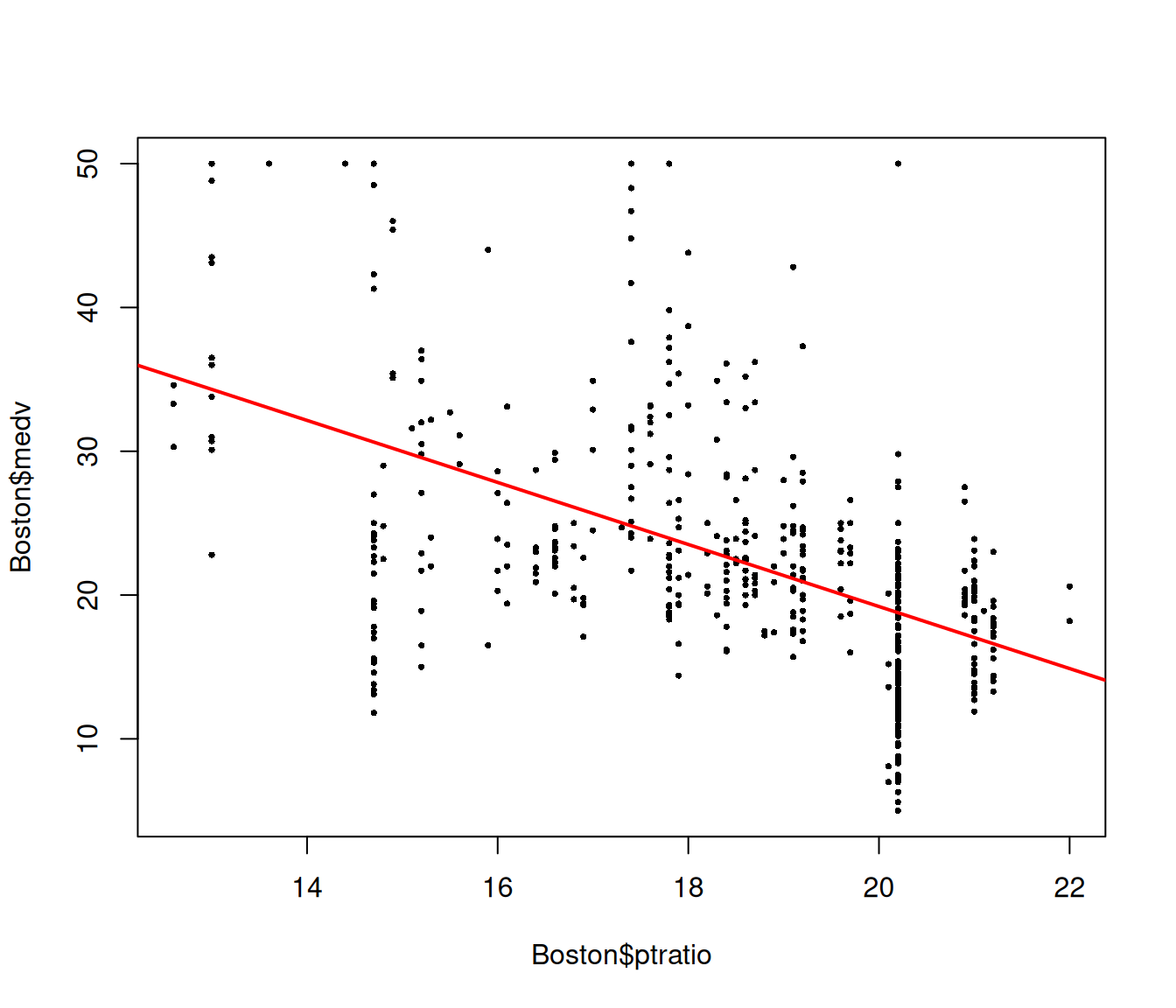
The summary method gives us more information on the univariate linear model we fit:
summary(lmfit)
#>
#> Call:
#> lm(formula = medv ~ ptratio, data = Boston)
#>
#> Residuals:
#>      Min       1Q   Median       3Q      Max
#> -18.8342  -4.8262  -0.6426   3.1571  31.2303
#>
#> Coefficients:
#>             Estimate Std. Error t value Pr(>|t|)
#> (Intercept)   62.345      3.029   20.58   <2e-16 ***
#> ptratio       -2.157      0.163  -13.23   <2e-16 ***
#> ---
#> Signif. codes:  0 '***' 0.001 '**' 0.01 '*' 0.05 '.' 0.1 ' ' 1
#>
#> Residual standard error: 7.931 on 504 degrees of freedom
#> Multiple R-squared:  0.2578, Adjusted R-squared:  0.2564
#> F-statistic: 175.1 on 1 and 504 DF,  p-value: < 2.2e-16
1.3 Multivariate linear regression
Univariate linear regression is almost always too simple of a model. For many phenomena, we expect the output to depend on several input variables. Multivariate linear regression (also known as ordinary least squares, or OLS) is a natural extension of univariate linear regression which allows us to fit a model with several variables.
Assume that there are \(p\) input variables, denoted \(x_1, \dots, x_p\), that our model can use to predict the output variable \(y\). The multivariate linear model has the form
\[y = \beta_0 + \beta_1 x_1 + \beta_2 x_2 + \dots + \beta_p x_p + \epsilon.\]
\(\beta_0, \dots, \beta_p\) are parameters of the model that we have to determine based on the data that we have. The model above can be written more succinctly as
\[y = \beta_0 + \mathbf{x}^\top \beta + \epsilon,\]
where \(\mathbf{x}^\top = \begin{pmatrix} x_1 & \dots & x_p \end{pmatrix}\) and \(\beta^\top = \begin{pmatrix} \beta_1 & \dots & \beta_p \end{pmatrix}\).1 For us, a vector such as \(\mathbf{x}\) is assumed to be a column vector.
Let \(n\) denote the number of observations in our dataset. For observation \(i\), let \(y_i\) denote the value of output variable and let \(\mathbf{x}_i\) denote the input features as a \(p\)-dimensional vector. We set our regression coefficients to be the values of \((\beta_0, \beta)\) which minimize the RSS:
\[(\hat\beta_0, \hat\beta) = \underset{(\beta_0, \beta) \in \mathbb{R}^{p+1}}{\text{argmin}} \; \sum_{i=1}^n \left[ y_i - (\beta_0 + \mathbf{x}_i^\top \beta) \right]^2. \tag{1.1}\]
Equation 1.1 can be written more succinctly with matrix notation. Let \(\mathbf{y}^\top = \begin{pmatrix} y_1 & \dots & y_n \end{pmatrix} \in \mathbb{R}^n\), and let \(\mathbf{X} \in \mathbb{R}^{n \times p}\) be the matrix such that its \(i\)th row is equal to \(\mathbf{x}_i\). We can rewrite Equation 1.1 as
\[(\hat\beta_0, \hat\beta) = \underset{(\beta_0, \beta) \in \mathbb{R}^{p+1}}{\text{argmin}} \; \|\mathbf{y} - \beta_0 \mathbf{1} - \mathbf{X} \beta \|_2^2, \tag{1.2}\]
where \(\mathbf{1}\) represents the \(n\)-dimensional vector of ones.
1.3.1 Fitting the OLS model
Fitting a multivariate linear model is easy in R. The code below fits an OLS model of medv against the ptratio and crim variables:
lmfit <- lm(medv ~ crim + ptratio, data = Boston)
summary(lmfit)
#>
#> Call:
#> lm(formula = medv ~ crim + ptratio, data = Boston)
#>
#> Residuals:
#>     Min      1Q  Median      3Q     Max
#> -17.851  -4.637  -1.051   2.582  32.246
#>
#> Coefficients:
#>             Estimate Std. Error t value Pr(>|t|)
#> (Intercept) 57.37835    2.98874  19.198  < 2e-16 ***
#> crim        -0.28142    0.04104  -6.857 2.06e-11 ***
#> ptratio     -1.83298    0.16305 -11.242  < 2e-16 ***
#> ---
#> Signif. codes:  0 '***' 0.001 '**' 0.01 '*' 0.05 '.' 0.1 ' ' 1
#>
#> Residual standard error: 7.592 on 503 degrees of freedom
#> Multiple R-squared:  0.3213, Adjusted R-squared:  0.3186
#> F-statistic: 119.1 on 2 and 503 DF,  p-value: < 2.2e-16
The code below fits an OLS model of medv against all the other variables in the Boston dataset:
lmfit <- lm(medv ~ ., data = Boston)
summary(lmfit)
#>
#> Call:
#> lm(formula = medv ~ ., data = Boston)
#>
#> Residuals:
#>     Min      1Q  Median      3Q     Max
#> -15.595  -2.730  -0.518   1.777  26.199
#>
#> Coefficients:
#>               Estimate Std. Error t value Pr(>|t|)
#> (Intercept)  3.646e+01  5.103e+00   7.144 3.28e-12 ***
#> crim        -1.080e-01  3.286e-02  -3.287 0.001087 **
#> zn           4.642e-02  1.373e-02   3.382 0.000778 ***
#> indus        2.056e-02  6.150e-02   0.334 0.738288
#> chas         2.687e+00  8.616e-01   3.118 0.001925 **
#> nox         -1.777e+01  3.820e+00  -4.651 4.25e-06 ***
#> rm           3.810e+00  4.179e-01   9.116  < 2e-16 ***
#> age          6.922e-04  1.321e-02   0.052 0.958229
#> dis         -1.476e+00  1.995e-01  -7.398 6.01e-13 ***
#> rad          3.060e-01  6.635e-02   4.613 5.07e-06 ***
#> tax         -1.233e-02  3.760e-03  -3.280 0.001112 **
#> ptratio     -9.527e-01  1.308e-01  -7.283 1.31e-12 ***
#> black        9.312e-03  2.686e-03   3.467 0.000573 ***
#> lstat       -5.248e-01  5.072e-02 -10.347  < 2e-16 ***
#> ---
#> Signif. codes:  0 '***' 0.001 '**' 0.01 '*' 0.05 '.' 0.1 ' ' 1
#>
#> Residual standard error: 4.745 on 492 degrees of freedom
#> Multiple R-squared:  0.7406, Adjusted R-squared:  0.7338
#> F-statistic: 108.1 on 13 and 492 DF,  p-value: < 2.2e-16
Some books drop the intercept term \(\beta_0\), since we can think of the intercept as the coefficient for an input variable that is always 1. We state the intercept term explicitly in this book as it is treated differently from the other parameters at times in the glmnet package.↩︎