26 Other regularized regression models
Thus far we have discussed elastic net models via the glmnet R package, and we hope that we’ve convinced you that they can meet many of your modeling needs. Nevertheless, we know that the elastic net is but one method in a prediction modelers toolbox, and it would be remiss if we didn’t talk about other penalized regression methods that we think you should know. In this chapter, we briefly highlight key penalized regression methods that we think you should be aware of and give pointers to their implementations.
26.1 Group lasso and group elastic net
The group lasso (Yuan and Lin 2005) and its elastic net extension is probably the most used penalized regression model following the elastic net. Consider using the group lasso in applications where your input features come in non-overlapping groups, and you either want the whole group to be included in the model or for the whole group to be excluded from the model.
Assume that the input features can be partitioned into \(K\) disjoint groups, and let \(\beta^{(k)}\) denote the coefficients corresponding to group \(k\). The relationship between the response and input features is modeled as
\[ y = \beta_0 + \beta_1 x_1 + \dots + \beta_p x_p, \]
and the coefficients are determined by the minimization problem
\[ \min_{\beta_0, \mathbf{\beta}} \quad \frac{1}{2n} \| \mathbf{y} - \beta_0 \mathbf{1} - \mathbf{X\beta} \|_2^2 + \lambda \sum_{k=1}^K \left[\alpha \|\beta^{(k)} \|_2 + \frac{1-\alpha}{2} \| \beta^{(k)} \|_2^2 \right]. \]
Please refer to Chapter 25 for an extended description of the group elastic net and the adelie package which has extremely efficient routines for fitting the group elastic net.
26.2 Sparse group lasso
The sparse group lasso (Simon et al. 2013) is an extension of the group lasso that gives sparsity both at the group level and within the group. For the sparse group lasso, the relationship between the response and input features is modeled as
\[ y = \beta_0 + \beta_1 x_1 + \dots + \beta_p x_p, \]
and the coefficients are determined by the minimization problem
\[ \min_{\beta_0, \mathbf{\beta}} \quad \frac{1}{2n} \| \mathbf{y} - \beta_0 \mathbf{1} - \mathbf{X\beta} \|_2^2 + \lambda \sum_{k=1}^K \left[(1-\alpha) \|\beta^{(k)} \|_2 + \alpha \| \beta^{(k)} \|_1 \right]. \]
We recommend the sparsegl R package (Liang et al. 2024) for fitting the sparse group lasso.
26.3 Overlapping group lasso
The group lasso assumes that the groups which the features come in are disjoint. There are some applications where the groups might overlap, meaning that some features belong to more than one group. (For example, in genetic association studies a gene might belong to more than one pathway.) The overlapping group lasso (Jacob et al. 2009) allows us to fit a model using the overlapping group information.
You can actually fit an overlapping group lasso model by using the original group lasso implementation: you just need to change the x matrix! What you have to do is “duplicate” features which appear in more than one group, then run the group lasso on the augmented data matrix.
This is best explained through an example. Assume that we have 5 features and our feature groups are \(\{1, 2, 3\}\) and \(\{2, 3, 4, 5\}\). Create a new input data matrix z with \(z_1 = x_1\), \(z_2 = x_2\), \(z_3 = x_3\), \(z_4 = x_2\), \(z_5 =x_3\), \(z_6=x_4\), \(z_7=x_5\). We then run the original group lasso with the z matrix and feature groups \(\{1, 2, 3\}\) and \(\{4, 5, 6, 7\}\).
26.4 hierNet
One limitation of the lasso is that it does not allow for interactions between the input features. hierNet (Bien et al. 2013) is a variation of the lasso that produces sparse interaction models that honor “hierarchy” restrictions (which we describe shortly).
hierNet models the response as
\[ y = \beta_0 + \sum_j \beta_j x_j + \frac{1}{2}\sum_{j \neq k} \Theta_{jk} x_j x_k, \]
where \(\Theta \in \mathbb{R}^{p \times p}\) satisfies \(\Theta = \Theta^\top\) and \(\Theta_{jj} = 0\) for all \(j\). In many settings, we want “hierarchy” to be enforced in our model, namely that an interaction effect is only allowed in the model if the corresponding main effects are also in the model. There are two commonly used hierarchical restrictions, which are probably best understood in math terms:
\[ \begin{aligned} \text{Strong hierarchy: } \quad &\widehat{\Theta}_{jk} \neq 0 \quad\Rightarrow\quad \hat{\beta}_j \neq 0 \text{ and } \hat{\beta}_k \neq 0, \\ \text{Weak hierarchy: } \quad &\widehat{\Theta}_{jk} \neq 0 \quad\Rightarrow\quad \hat{\beta}_j \neq 0 \text{ or } \hat{\beta}_k \neq 0. \end{aligned} \]
hierNet has the ability to fit models with either strong hierarchy or weak hierarchy. hierNet is implemented in the hierNet R package.
26.5 glinternet
Similar to hierNet, glinternet (Lim and Hastie 2015) was introduced as a way for learning pairwise interactions in a linear regression or logistic regression model. There are two main differences between glinternet and hierNet:
- glinternet works out-of-the-box for categorical variables (and can handle a mix of categorical and continuous variables), whereas hierNet only works for continuous variables1.
- glinternet can only enforce strong hierarchy, whereas hierNet can enforce either strong or weak hierarchy.
glinternet is implemented in the glinternet R package.
26.6 UniLasso
The UniLasso (Chatterjee et al. 2025) is a variant of the lasso that has greater model stability and interpretability. The uniLasso ensures that:
- The signs of the final coefficients agree with the signs of the univariate coefficients (or they are zero); and
- Features with larger univariate coefficients will tend to have larger coefficients in the final model.
UniLasso is implemented in the uniLasso R package.
26.7 Cooperative learning and multiview analysis
In some applications we have collected datasets from many different sources and are interested in using them in combination to predict an outcome of interest. For example, in biomedicine we have data from genomics, epigenomics, transcriptomics, proteomics, and metabolomics, just to name a few sources.
There are many ways to “fuse” the data across sources. Broadly speaking they fall into two categories:
- Early fusion: Tranform the multiple data views into a single representation before feeding it into a supervised learning model.
- Late fusion: Build individual models for distinct data views, then combine these predictions into a single final predictor.
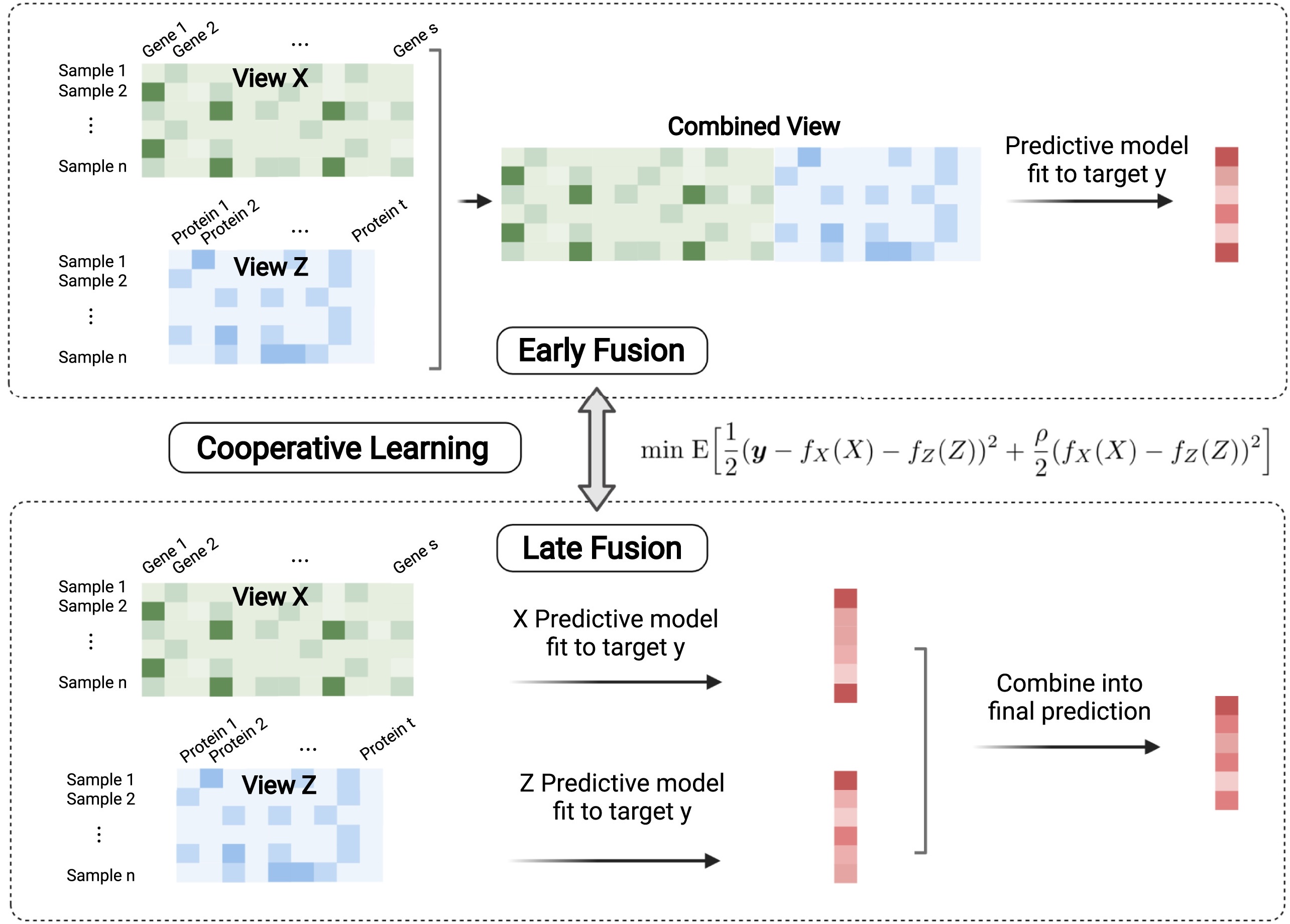
Cooperative learning (Ding et al. 2022) is a supervised learning algorithm that encompasses both early and late fusion, as well as blended versions of these methods. It encourages the predictions from different views to agree and chooses the degree of agreement in a data-adaptive manner.
Cooperative learning is implemented in the multiview R package.
26.8 Pretraining and the lasso
Pretraining is a popular and powerful paradigm in machine learning to pass information from one model to another. We start with a model that has been trained on a large corpus of data, then fine-tune the model on a smaller dataset. We only care about the model’s performance on the smaller dataset. Instead of training a model from scratch on the smaller dataset, we start with the pretrained model with the hope of using information from the large corpus of data to guide our fine-tuned model to better performance.
Craig et al. (2024) proposes a way to do this with the lasso. [TODO Erin could you fill in the details here? Since you wrote the paper :)]
This pretraining framework is implemented in the ptLasso R package.
26.9 Graphical lasso
Strictly speaking the graphical lasso (Friedman et al. 2007) is not a supervised learning method, but we think it is interesting and important enough that we include it in this list.
The graphical lasso deals with the problem of estimating sparse undirected graphical models from data. Assume that we have \(n\) multivariable normal observations of dimension \(p\), with unknown mean \(\mu\) and unknown covariance matrix \(\Sigma\). The inverse of the covariance matrix (also known as the precision matrix), \(\Theta = \Sigma^{-1}\), has the property that if \(\Theta_{ij} = 0\), then variables \(i\) and \(j\) are conditionally independent, given the other variables. Hence, estimating the precision matrix is equivalent to estimating the conditional independence graph between the variables.
If \(S\) is the empirical covariance matrix, the graphical lasso problem is to maximize the penalized log-likelihood
\[ \log \det \Theta - \text{tr}(S \Theta) - \rho \| \Theta \|_1 \]
over non-negative definite matrices \(\Theta\). In the above, \(\rho \geq 0\) is a tuning parameter, just like \(\lambda\) for the lasso. Larger \(\rho\) values correspond to sparser conditional independence graphs.
The graphical lasso is implemented in the glasso R package.
While one could use one-hot encoding to convert categorical variables into a set of continuous variables, the resulting interactions between these new variables might not make much sense.↩︎