library(survival)

# create data
set.seed(1)
nobs <- 100; nvars <- 15
x <- matrix(rnorm(nobs * nvars), nrow = nobs)
ty <- rep(rexp(nobs / 5), each = 5)
tcens <- rbinom(n = nobs, prob = 0.3, size = 1)
y <- Surv(ty, tcens)

head(y)
#> [1] 0.6046991+ 0.6046991+ 0.6046991+ 0.6046991+ 0.6046991+ 0.816112612 Cox regression
12.1 What is survival analysis?
Survival analysis is a branch of statistics that focuses on modeling the time until an event of interest occurs. Some examples of events of interest are death, disease progression, equipment failure, and customer churn.
12.1.1 Survival data
A key difference between survival analysis and supervised learning is the data we have available to us. In survival analysis, instead of \(y_i \in \mathbb{R}\) as a response, we have \((y_i, \delta_i) \in \mathbb{R}_+ \times \{ 0, 1\}\). Here, \(y_i\) is the observed time for observation \(i\). \(\delta_i\) is the censoring indicator for observation \(i\):
\(\delta_i = 1\) if \(y_i\) is the failure time, and
\(\delta_i = 0\) if \(y_i\) is the right-censoring time.
For example, if the event of interest is death, \((y_i, \delta_i) = (5, 1)\) means that subject \(i\) died at time 5. On the other hand, \((y_i, \delta_i) = (5, 0)\) means that subject \(i\) was still alive at time 5, and all we can say is that subject \(i\)’s time of death is \(\geq 5\).
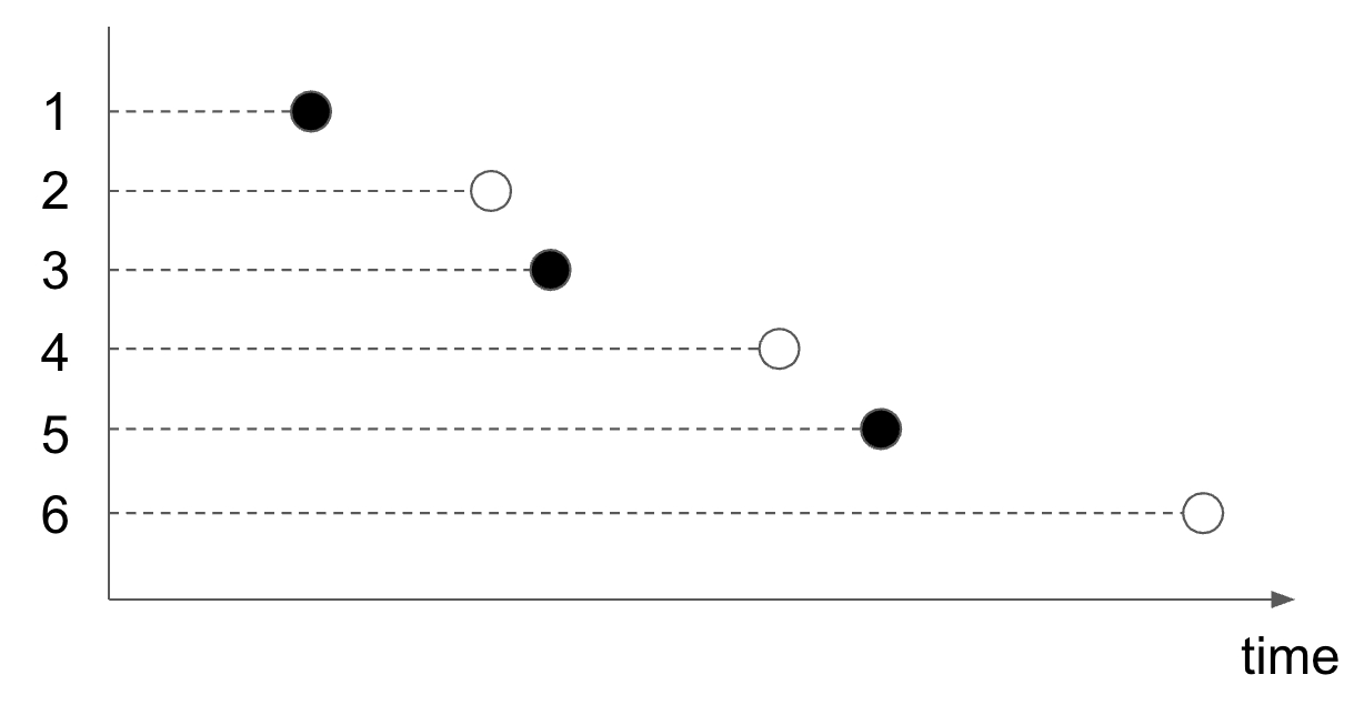
The figure below is one way to visualize survival data. We order the observations in increasing order of time (\(y_i\)). A black dot indicates that a failure was observed (\(\delta_i = 1\)), while a white dot indicates that a failure was not observed (\(\delta_i = 0\)).
12.1.2 Key quantities in survival analysis
Survival analysis also differs from supervised learning in the quantities that we seek to estimate. The first key quantity we want to estimate is the survival function \(S(\cdot)\), which is the probability that an individual survives beyond time \(t\):
\[S(t) = P (T > t).\]
A common non-parametric method for estimating \(S\) from censored data is the Kaplan-Meier Estimator:
\[\widehat{S}(t) = \prod_{i: t_i \leq t} \left( 1 - \dfrac{d_i}{n_i}\right),\]
where \(t_i\) is a time when at least one event happened, \(d_i\) is the number of events that happened at time \(t_i\), and \(n_i\) is the number of observations in the dataset which are known to have survived up to time \(t_i\) (i.e. have not yet had an event or have been censored).
Let’s compute the Kaplan-Meier estimator for our example data below:
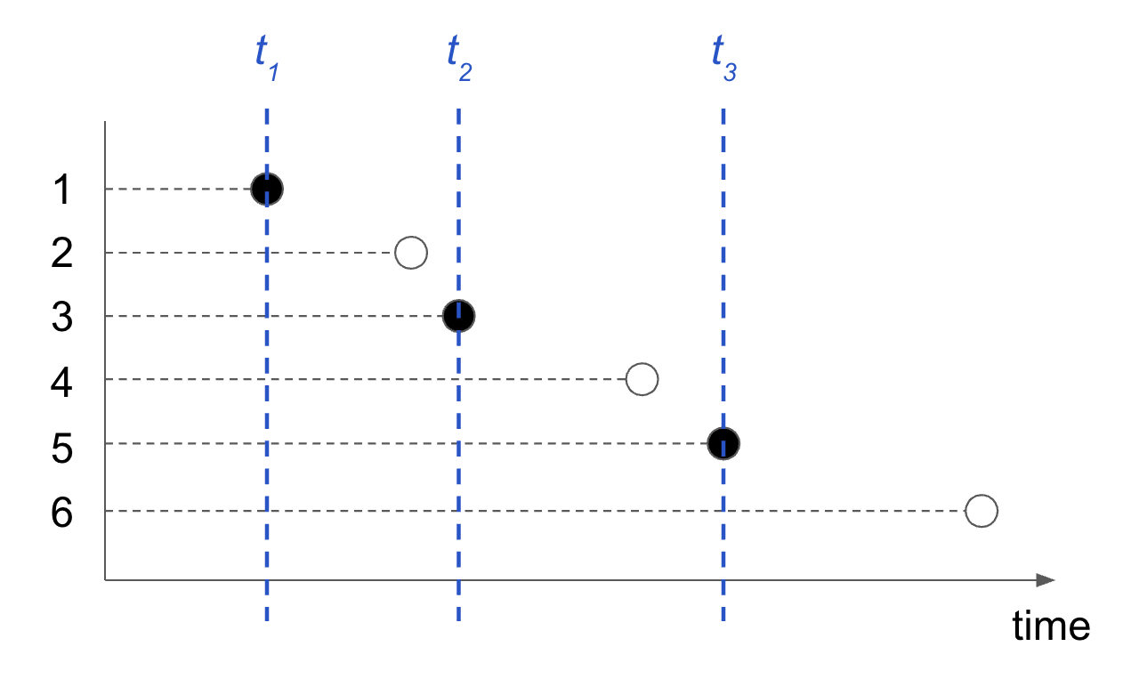
- For \(t < t_1\), \(\widehat{S}(t) = 1\) since no event has happened yet.
- For \(t_1 \leq t < t_2\), \(\widehat{S}(t) = 1 - \frac{1}{6}\).
- For \(t_2 \leq t < t_3\), \(\widehat{S}(t) = (1 - \frac{1}{6})(1 - \frac{1}{4})\).
- For \(t_3 \leq t\), \(\widehat{S}(t) = (1 - \frac{1}{6})(1 - \frac{1}{4})(1 - \frac{1}{2})\).
A related quantity that is estimated in many applications instead of the survival function is the hazard function \(h(\cdot)\), defined by
\[h(t) = \lim_{\Delta t \rightarrow 0} \frac{P(t \leq T < t + \Delta t \;|\; T \geq t)}{\Delta t}.\]
If the survival function \(S\) is differentiable, the hazard function is
\[h(t) = - \dfrac{d}{dt} \log S(t).\]
We care about the hazard function because it is the instantaneous risk of experiencing the event at time \(t\), and hence describes how the risk of the event changes over time.
12.2 The Cox proportional hazards model
The Cox proportional hazards model (Cox 1972), often referred to simply as the Cox model, is a commonly used model for the relationship between the predictor variables and survival time. It assumes a semi-parametric form for the hazard function
\[h_i(t) = h(t) e^{\mathbf{x}_i^\top \beta},\]
where \(h_i(t)\) is the hazard for observation \(i\) at time \(t\), \(h\) is the baseline hazard for the entire population of observations, and \(\beta \in \mathbb{R}^p\) is the vector of coefficients to be estimated.
Let \(t_1 < \dots < t_m\) denote the unique failure times and let \(j(i)\) denote the index of the observation failing at time \(t_i\). (Assume for the moment that the \(y_i\)’s are unique.) If \(y_j \geq t_i\), we say that observation \(j\) is at risk at time \(t_i\). Let \(R_i\) denote the risk set at time \(t_i\), i.e. the set of observations which are at risk at time \(t_i\). The partial likelihood1 is defined as
\[L(\beta) = \prod_{i=1}^m \dfrac{\exp \left( \mathbf{x}_{j(i)}^\top \beta \right)}{\sum_{j\in R_i} \exp \left( \mathbf{x}_j^\top \beta \right)}. \tag{12.1}\]
The partial likelihood is the conditional likelihood that the failure occurs for observation \(j(i)\) given all the observations at risk. The partial likelihood is a fairly complicated object, so we demonstrate how to compute it on a simple example. First, let \(s_j = \exp \left( \mathbf{x}_j^\top \beta \right)\) so that Equation 12.1 can be written more succinctly as
\[L(\beta) = \prod_{i=1}^m \dfrac{ s_{j(i)}}{\sum_{j\in R_i} s_j }.\]
Consider the data below:
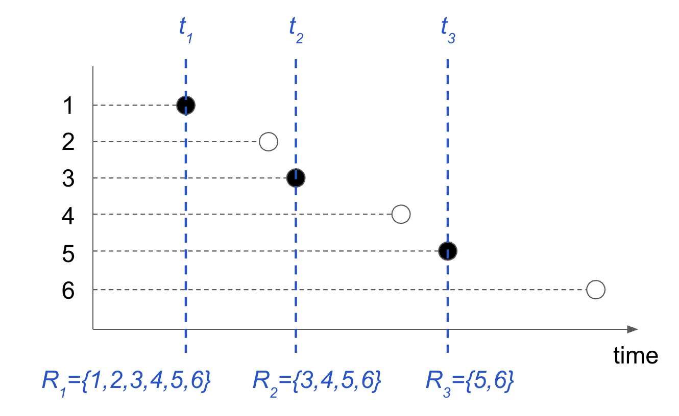
There are 3 unique failure times, and the risk sets associated with each failure time is indicated in the figure. The partial likelihood for this data is
\[L(\beta) = \left( \dfrac{s_1}{s_1 + s_2 + s_3 + s_4 + s_5 + s_6} \right) \left( \dfrac{s_3}{s_3 + s_4 + s_5 + s_6} \right) \left( \dfrac{s_5}{s_5 + s_6} \right).\]
The coefficient vector \(\beta\) in the Cox model is estimated by maximizing the partial likelihood. This is equivalent to minimizing the negative log partial likelihood
\[-\ell(\beta)=\frac{2}{n} \sum_{i=1}^m \left[ -\mathbf{x}_{j(i)}^\top \beta + \log \left( \sum_{j \in R_i} e^{\mathbf{x}_j^\top \beta} \right) \right]. \tag{12.2}\]
The beauty of this approach is that it allows the estimation of \(\beta\) (how different variables affect the survival rate) while ignoring the baseline hazard rate \(h(t)\).
12.3 The regularized Cox model
For classical problems, with many more observations \(n\) than predictors \(p\), the Cox model performs well. However, in problems with \(p > n\), we get degenerate behavior: to maximize the partial likelihood, all of the \(\beta_i\)’s are sent to \(\pm \infty\).
To combat this issue, Simon et al. (2011) proposed an elastic net regularization path version of the Cox model:
\[\hat\beta = \underset{\beta \in \mathbb{R}^p}{\text{argmin}} \; \left[ -\ell(\beta) + \lambda \left(\frac{1-\alpha}{2}\|\beta \|_2^2 + \alpha \|\beta \|_1 \right) \right].\]
We can fit the regularized Cox model with the glmnet package by specifying family="cox". As with other models we’ve seen, the input features can be passed as an \(n \times p\) matrix. The recommended approach for preparing the response variable for glmnet is to use the output of a call to Surv from the survival package (Therneau 2022).
Fit the regularized Cox model by calling glmnet with family = "cox"2:
# fit the regularized Cox model
fit <- glmnet(x, y, family = "cox", cox.ties = "breslow")
fit
#>
#> Call:  glmnet(x = x, y = y, family = "cox", cox.ties = "breslow")
#>
#>    Df  %Dev   Lambda
#> 1   0  0.00 0.129100
#> 2   1  0.40 0.117600
#> 3   1  0.74 0.107200
#> 4   1  1.02 0.097670
#> 5   1  1.25 0.088990
#> 6   3  1.64 0.081080
....
For backward compatibility, glmnet can also accept a two-column matrix with column names "time" and "status" for right-censored data. The columns must be "time" indicating the failure/censoring times, and "status" which is 1 if the time is a failure time, and 0 if it is a censoring time. The code below demonstrates fitting the regularized Cox model with such an input format.
library(knitr)
ymat <- cbind(time = ty, status = tcens)
kable(head(ymat))| time | status |
|---|---|
| 0.6046991 | 0 |
| 0.6046991 | 0 |
| 0.6046991 | 0 |
| 0.6046991 | 0 |
| 0.6046991 | 0 |
| 0.8161126 | 1 |
….
# fit the regularized Cox model
matfit <- glmnet(x, ymat, family = "cox", cox.ties = "breslow")
matfit
#>
#> Call:  glmnet(x = x, y = ymat, family = "cox", cox.ties = "breslow")
#>
#>    Df  %Dev   Lambda
#> 1   0  0.00 0.129100
#> 2   1  0.40 0.117600
#> 3   1  0.74 0.107200
#> 4   1  1.02 0.097670
#> 5   1  1.25 0.088990
#> 6   3  1.64 0.081080
....
As with earlier models, the returned object here has a coef method for obtaining coefficients at specific \(\lambda\) values, as well as a plot method for plotting the coefficient profile of the model across \(\lambda\) values.
12.3.1 Ties in survival times
If our data contains tied observed times, glmnet handles them through the cox.ties argument, which selects between the Breslow (Breslow 1972) and Efron (Efron 1977) approximations of the partial likelihood; it then maximizes the elastic net-regularized version of the chosen approximation. This argument was introduced in glmnet 5.x—earlier versions supported only the Breslow approximation. The current default is Breslow, though this is expected to change to Efron in a future release. By contrast, the coxph function in the survival package defaults to the Efron approximation. To compare survival::coxph with an unpenalized Cox model from glmnet (i.e. \(\lambda = 0\)), make the tie handling match on both sides—for example, set ties = "breslow" in the coxph call together with cox.ties = "breslow" in glmnet (the current default), or use "efron" in both.
12.4 Cross-validation for Cox models
The cv.glmnet function can be used to perform \(K\)-fold cross-validation (CV) for the Cox model. This works like CV for other model families, with two main differences.
First, for Cox models the possible values for type.measure (loss to use for CV) are "deviance" (default) and "C", which uses the Harrell C-index. This is a concordance measure like the area under the curve (AUC) measure that we use for binary data, except we only use pairs whose times we can actually compare. For right-censored data, if an observation is right-censored at a time before another observation’s death time, they are not comparable (we don’t know which death time would have come first), and so we exclude these pairs from the C-index computation.
Second, the option grouped = TRUE (default) obtains the CV partial likelihood for the \(k\)th fold by subtraction, i.e. by subtracting the log partial likelihood evaluated on the full dataset from that evaluated on the dataset excluding the \(k\)th fold. This makes more efficient use of risk sets. With grouped = FALSE the log partial likelihood is computed only on the \(k\)th fold, which is only reasonable if each fold has a large number of observations.
12.5 Plotting survival curves
The beauty of the Cox partial likelihood is that the baseline hazard, \(h(t)\), is not required for inference on the model coefficients \(\beta\). However, the estimated hazard is often of interest to users. The survival package already has a well-established survfit method that can produce estimated survival curves from a fitted Cox model. Glmnet implements a survfit method for regularized Cox models fit by glmnet by creating the coxph object corresponding to the model and calling survival::survfit.
To be consistent with other methods in glmnet, if the s parameter is not specified, survival curves are returned for the entire lambda sequence as a list, one element for each lambda value. The code below demonstrates this:
sf <- survival::survfit(fit, x = x, y = y)
length(sf)          # number of returned survival curves
#> [1] 50
length(fit$lambda)  # number of lambda values
#> [1] 50
A more typical use is to plot the survival curve for a specific value of the \(\lambda\) tuning parameter. The code below is an example of calling survfit for coxnet objects for a particular value of \(\lambda\). Note that we had to pass the original model matrix x and response y to the survfit call: they are needed for survfit.coxnet to reconstruct the required coxph object. The survival curves are computed for the individuals represented in newx: we get one curve per individual, as seen in the figure below. (We are unable to provide standard errors for these survival curves, so we do not present the confidence bounds for them.)
sf_obj <- survfit(fit, s = 0.05, x = x, y = y, newx = x[1:2, ])
plot(sf_obj, col = 1:2, mark.time = TRUE, pch = "12")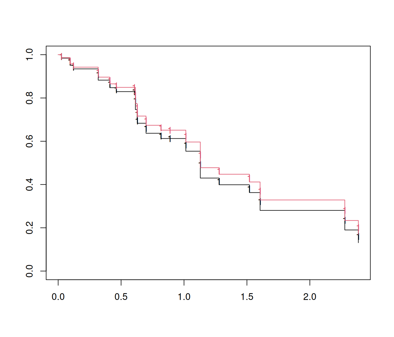
Note
Don’t forget to specify newx! Not specifying newx will not throw an error. However, if newx is not specified, a survival curve is produced for a single “pseudo” subject with covariate values equal to the means of the data set, and this resulting curve almost never makes sense.
The survfit method is available for Cox models fitted by cv.glmnet as well. By default, the survival curves are computed for the lambda.1se value of the \(\lambda\) hyperparameter. The user can use the code below to compute the survival curve at the lambda.min value:
# fit cv.glmnet model
set.seed(1)
cfit <- cv.glmnet(x, y, family = "cox", cox.ties = "breslow", nfolds = 5)

# compute and plot survival curve
sf_obj <- survfit(cfit, s = "lambda.min", x = x, y = y, newx = x[1:2, ])
plot(sf_obj, col = 1:2, mark.time = TRUE, pch = "12")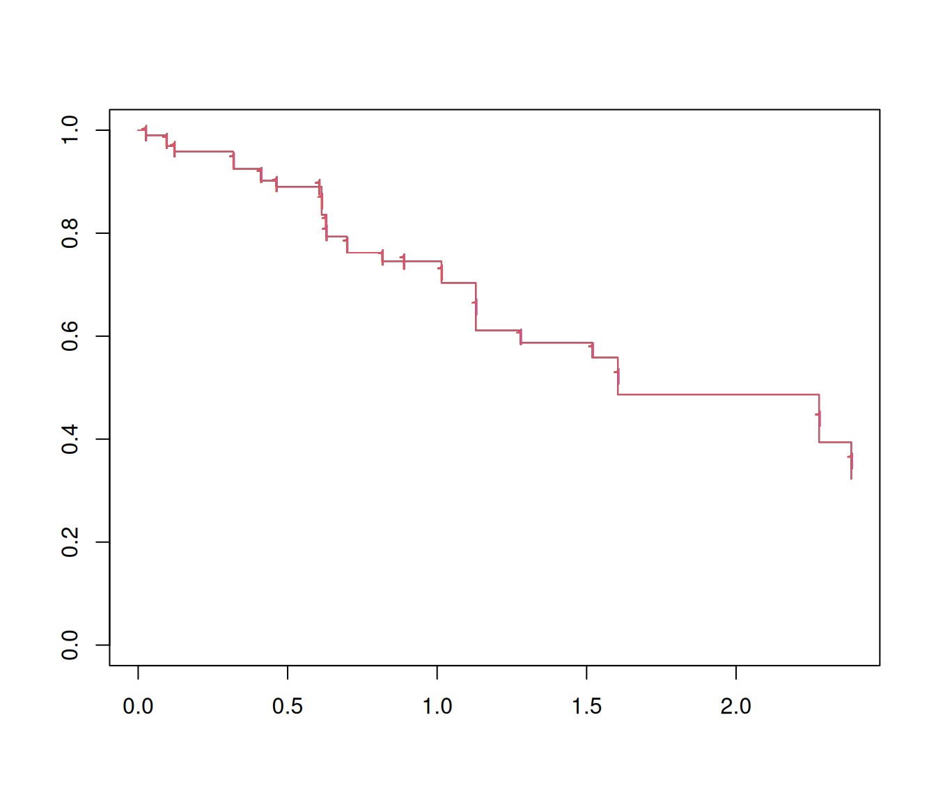
12.6 Additional notes
For algorithmic details on how we solve the minimization problem for the elastic net Cox regression model efficiently, see Simon et al. (2011). For details on handling ties see computations for partial likelihood at the glmnet homepage.
Note that the exponent does not include an intercept term. If we replace \(\mathbf{x}_{j(i)}^\top \beta\) with \(\beta_0 + \mathbf{x}_{j(i)}^\top \beta\), \(\exp(\beta_0)\) appears in both the numerator and denominator of each term in the partial likelihood. Hence, we can assume that \(\beta_0 = 0\) without loss of generality.↩︎
Starting with glmnet 5.x, both the Efron and Breslow methods for handling tied event times are available through the
cox.tiesargument. The current default is"breslow", but"efron"(which matchessurvival::coxph) is expected to become the default in a future release. To lock in the present behavior and avoid the accompanying deprecation message, we passcox.ties = "breslow"explicitly throughout this book; passcox.ties = "efron"to use the Efron approximation instead.↩︎