data("CoxExample")
x <- CoxExample$x
y <- CoxExample$y
strata <- c(rep(1, 500), rep(2, 500))
y2 <- stratifySurv(y, strata)
str(y2)
#>  'stratifySurv' num [1:1000, 1:2]  1.76878   0.54528   0.04486+  0.85032+  0.61488   0.29861+  0.01717+ 15.97135   0.64802   1.91448+ ...
#>  - attr(*, "dimnames")=List of 2
#>   ..$ : NULL
#>   ..$ : chr [1:2] "time" "status"
#>  - attr(*, "type")= chr "right"
#> - attr(*, "strata")= num [1:1000] 1 1 1 1 1 1 1 1 1 1 ...13 Stratified Cox models
An extension of the Cox model is to allow for strata. These strata divide the units into disjoint groups, with each group having its own baseline hazard function but having the same coefficient values \(\beta\). Specifically, if the units are divided into \(K\) strata, then the stratified Cox model assumes that a unit in stratum \(k\) has the hazard function
\[h_i(t)=h_k(t) e^{\mathbf{x}_i^\top \beta},\]
where \(h_k(t)\) is the shared baseline hazard for all units in stratum \(k\).
In several applications, allowing different subgroups to have different baseline hazards approximates reality more closely. For example, it might be reasonable to have different baseline hazards based on gender in clinical trials, or a separate baseline for each center in multi-center trials.
While this gives the model a lot more flexibility, inference for the Cox model actually doesn’t change much at all! For each stratum \(k\), its partial likelihood \(L_k(\beta)\) is as in Equation 12.1, except (i) we only consider failure times for observations from stratum \(k\), and (ii) we only consider observations from stratum \(k\) in the determination of the risk sets. The partial likelihood for the entire dataset is simply the product of the partial likelihoods of the strata:
\[L(\beta) = \prod_{k=1}^K L_k(\beta).\]
Let’s illustrate this with an example. Consider this example we presented in dataset Chapter 12:
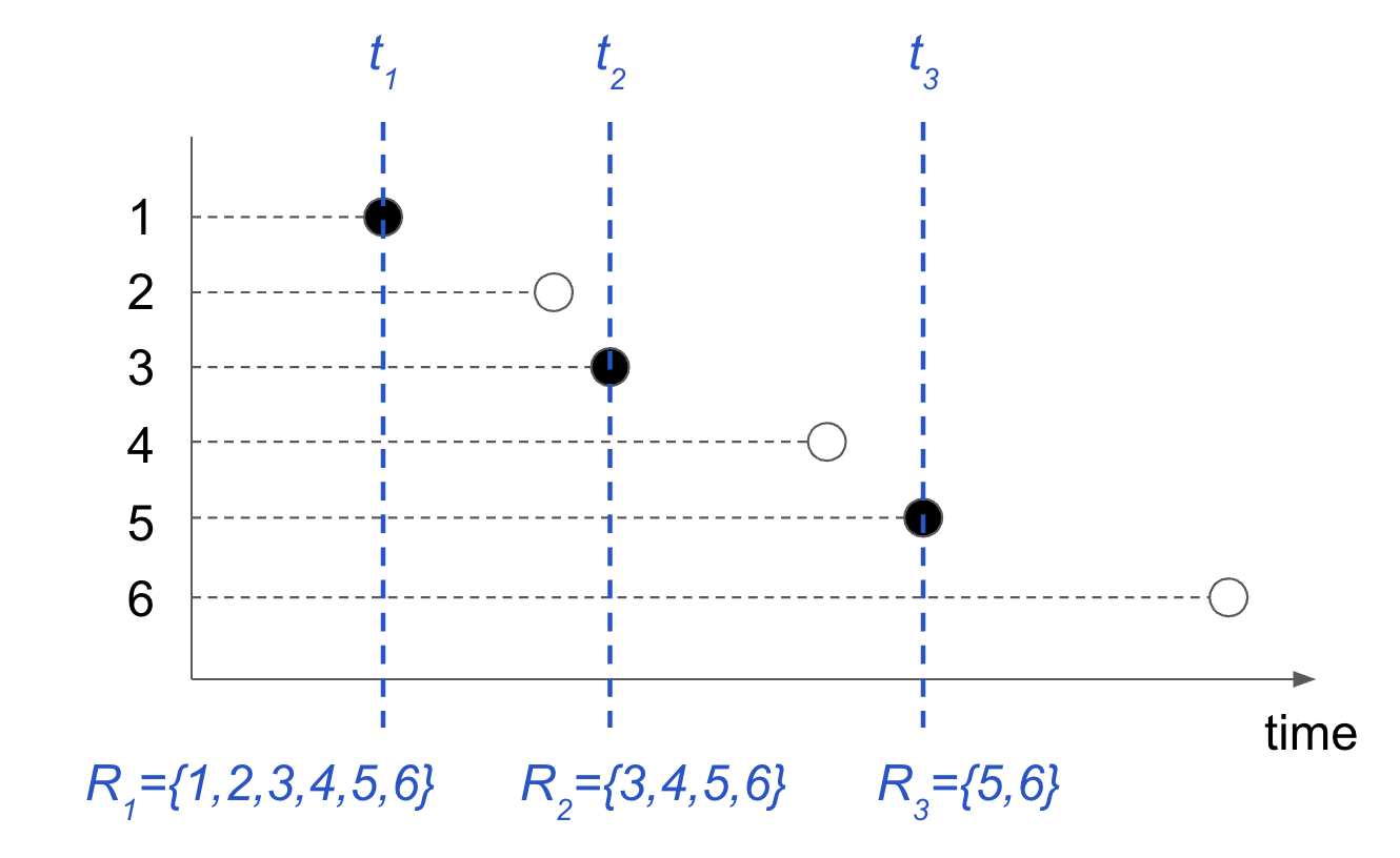
Without strata, the partial likelihood for this data is
\[L(\beta) = \left( \dfrac{s_1}{s_1 + s_2 + s_3 + s_4 + s_5 + s_6} \right) \left( \dfrac{s_3}{s_3 + s_4 + s_5 + s_6} \right) \left( \dfrac{s_5}{s_5 + s_6} \right),\] where we used the shorthand \(s_j = \exp \left( \mathbf{x}_j^\top \beta \right)\). Now, assume that observations 1, 2 and 4 belong to stratum 1 while observations 3, 5 and 6 belong to stratum 2. The figure below illustrates the split as well as the updated risk sets.
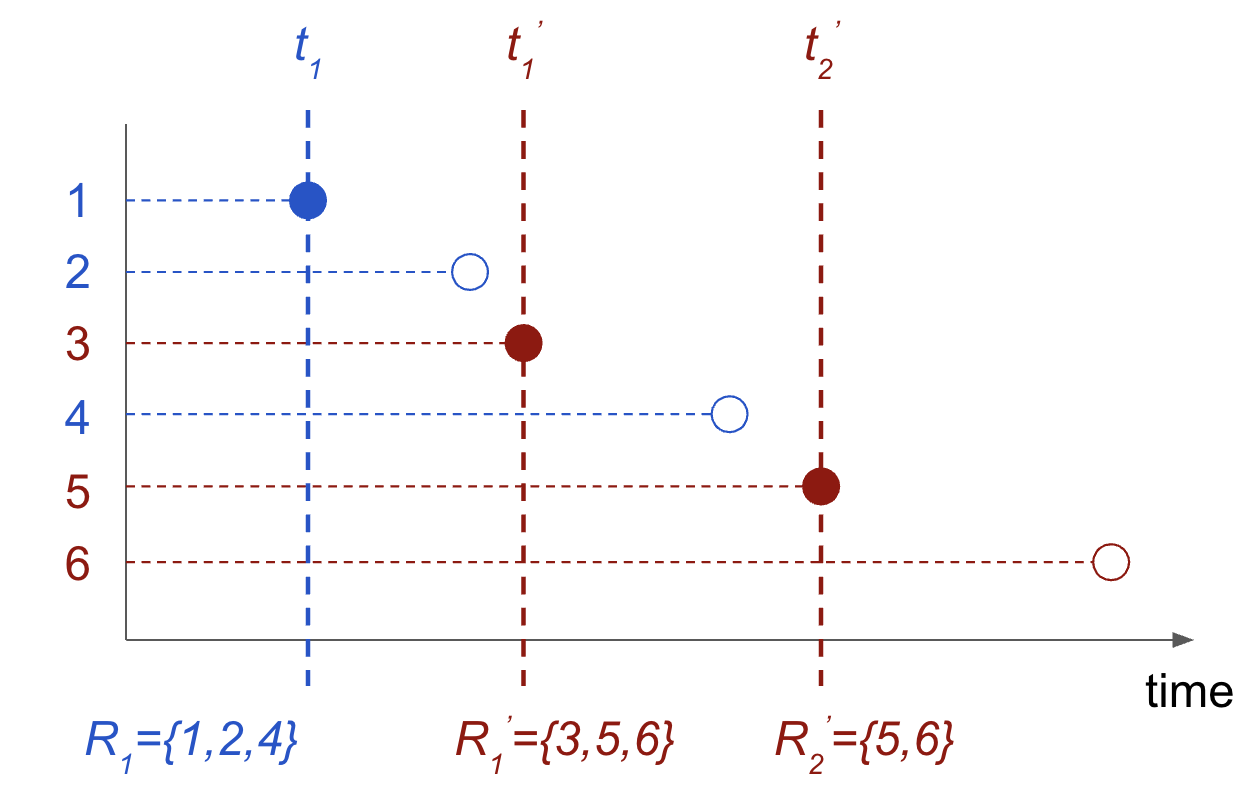
Based on these risk sets, the partial likelihoods for the strata are
\[\begin{aligned} L_1(\beta) &= \left( \frac{s_1}{s_1 + s_2 + s_4} \right), \\ L_2(\beta) &= \left( \frac{s_3}{s_3 + s_5 + s_6} \right) \left( \frac{s_5}{s_5 + s_6} \right), \end{aligned}\]
and the partial likelihood for the entire dataset is \(L(\beta) = L_1(\beta) L_2(\beta)\).
As with the Cox model without strata, instead of maximizing the partial likelihood we minimize the negative log partial likelihood:
\[\ell(\beta) = \sum_{k=1}^K \ell_k(\beta),\]
where \(\ell_k(\beta)\) is defined as in Equation 12.2, but considering just the units in stratum \(k\).
13.1 Fitting the stratified Cox model
To fit an unpenalized stratified Cox model, the survival package (Therneau 2022) has a special strata function that allows users to specify the strata variable in formula syntax. Since glmnet does not work with formulas, we needed a different approach for specifying strata. To fit regularized stratified Cox models with glmnet, the user needs to add a strata attribute to the response y. glmnet checks for the presence of this attribute and if it is present, it fits a stratified Cox model. We note that the user cannot simply add the attribute manually because R drops attributes when subsetting vectors. Instead, the user should use glmnet’s stratifySurv function to add the strata attribute. (stratifySurv creates an object of class "stratifySurv" that inherits from the class "Surv", ensuring that glmnet can reassign the strata attribute correctly after any subsetting.)
The code below shows an example of how to fit a regularized stratified Cox model with glmnet; there are a total of 1,000 observations, with the first 500 belonging to the first strata and the rest belonging to the second strata. We first prepare the response variable with a call to stratifySurv:
We then fit the model with glmnet (or cv.glmnet with the stratifySurv object as the response variable.
fit <- glmnet(x, y2, family = "cox", cox.ties = "efron")
fit
#>
#> Call:  glmnet(x = x, y = y2, family = "cox", cox.ties = "efron")
#>
#>    Df %Dev   Lambda
#> 1   0 0.00 0.235500
#> 2   2 0.23 0.214600
#> 3   3 0.69 0.195500
#> 4   3 1.19 0.178200
#> 5   4 1.63 0.162300
#> 6   4 2.13 0.147900
#> 7   4 2.55 0.134800
#> 8   4 2.90 0.122800
#> 9   6 3.20 0.111900
#> 10  6 3.56 0.101900
#> 11  8 3.90 0.092890
....
13.2 Plotting for stratified Cox models
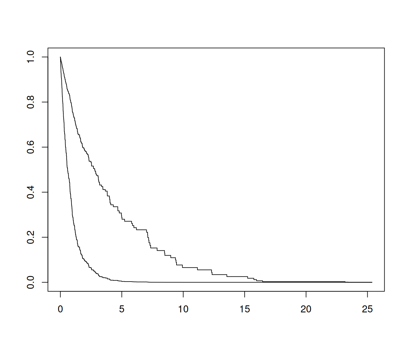
If the original model was fit with strata, we need to specify the strata for the observations when plotting the survival curves with survfit. We do this via the newstrata argument.
# survival curve plot for first two individuals in dataset
plot(survival::survfit(fit, s = 0.01, x = x, y = y2,
                       newx = x[1:2, ], newstrata = strata[1:2]))