| set | patients | features | deaths |
|---|---|---|---|
| discovery | 997 | 754 | 487 |
| validation | 983 | 754 | 478 |
| total | 1980 | 754 | 965 |
27 Predicting molecular breast cancer subtypes from the METABRIC data
We study the problem of classifying breast cancer subtypes in the publicly available METABRIC breast cancer data (cBioPortal for Cancer Genomics, n.d.), a good example of fitting multiclass and binary reponse models with glmnet. The data contains gene expression (GEX) and copy number variation (CNV) on a discovery and a validation set of samples. Curtis et al. (2012) had used an integrative clustering on the GEX and CNV discovery set to obtain 10 clusters, and then assessed reproducibility of the cluster classification on the validation set using a Nearest Shrunken Centroids (NSC) classifier. Three metrics were used: similar proportions of cases in clusters, similar hazard ratios between the discovery and validation sets, and the in-group proportions measure. Lazarov and Tibshirani (2026) analyze the same data using LASSO classifiers shown below using glmnet along with pamr to reproduce the NSC classifier clusterings.
| model | description |
|---|---|
| ungrouped multinomial | cv.glmnet(family = "multinomial", type.multinomial = "ungrouped") |
| grouped multinomial | as above with type.multinomial = "grouped" |
| one-versus-rest (OVR) | ten separate binomial lassos, one per cluster |
pamr |
nearest shrunken centroids (Tibshirani et al. 2002) |
The classification task here is unusual as there are no “ground truth” labels in the validation set; instead the validation set survival data is to assess prediction accuracy.
The data is downloadable from METABRIC cBioPortal and requires some processing per code in Section 27.5 to obtain the dat object containing discovery and validation data in what follows. Here is a data summary.
The 754 features are 39 copy-number and 715 expression probes with no missing values.
| 1 | 2 | 3 | 4 | 5 | 6 | 7 | 8 | 9 | 10 |
|---|---|---|---|---|---|---|---|---|---|
| 76 | 45 | 156 | 167 | 94 | 44 | 109 | 143 | 67 | 96 |
27.1 Fitting the four models
Before fitting, we assign samples to folds once for a clear comparison among the models.
x <- dat$discovery$x
y <- dat$discovery$y
n <- nrow(x)
set.seed(42L)
## 100 copies of each fold label and select exactly n to match Discovery sample size
foldid <- sample(rep(seq_len(10), trunc(n / 10) + 1L))[seq_len(n)]
The two multinomial fits below differ only in type.multinomial, which decides how a gene’s ten class coefficients are penalized:
"ungrouped"penalizes each of the ten separately, so a gene may enter the model for one cluster and stay out of the rest — here the per-cluster supports run from 7 genes (cluster 6) to 64 (cluster 4), 267 distinct genes in all,"grouped"applies a group-lasso penalty to the ten coefficients jointly, so a gene is either selected for every cluster or dropped altogether, yielding one shared signature of 234 genes. The argumentkeep = TRUEretains the pre-validated predictions we will need later for per-cluster error.
cv_ungrouped <- cv.glmnet(x, y, family = "multinomial",
                          type.multinomial = "ungrouped",
                          type.measure = "class", foldid = foldid, keep = TRUE)
cv_grouped   <- cv.glmnet(x, y, family = "multinomial",
                          type.multinomial = "grouped",
                          type.measure = "class", foldid = foldid, keep = TRUE)
The OVR arm is ten binomial lassos, each with its own lambda.min. Note the two separate steps: each model is scored on its own binomial error, but a patient is labeled by comparing all ten probabilities.
ovr <- lapply(clusters, function(k) {
  cv.glmnet(x, as.integer(y == k), family = "binomial",
            type.measure = "class", foldid = foldid, keep = TRUE)
})

## one label per patient: the cluster whose binomial gives the highest probability
## each predict() returns an n x 1 matrix, so cbind gives n patients x 10 clusters
p <- do.call(cbind, lapply(ovr, predict, newx = newx, s = "lambda.min",
                           type = "response"))
labels <- factor(clusters[max.col(p, ties.method = "first")], levels = clusters)
27.2 Cross-validated error and sparsity
The table below shows the obtained CV errors and number of features for each model.
| model | cv error | no. of features |
|---|---|---|
| ungrouped | 0.1374 | 267 |
| grouped | 0.1063 | 234 |
| ovr | 0.0572 | 401 |
| pamr | 0.0822 | 754 |
The pamr row is a reference, against which we assess the others. The multinomial models are comparable in terms of error, but pick the smallest number of features. OVR, on the other hand, has the smallest error, but the number of features chosen is closer to those of multinomial models than pamr.
The lasso models yield real gains in sparsity: their feature sets are much smaller than pamr which retains all 754 genes at its chosen threshold; the glmnet models use a few hundred, and the ungrouped and OVR fits use very few for some clusters — 7 genes for cluster 6, 9 for cluster 2. So for an oncologist a shorter list of genes that may define a subtype is welcome as it aids interpretability and might suggest further paths for research.
27.3 Overall Survival
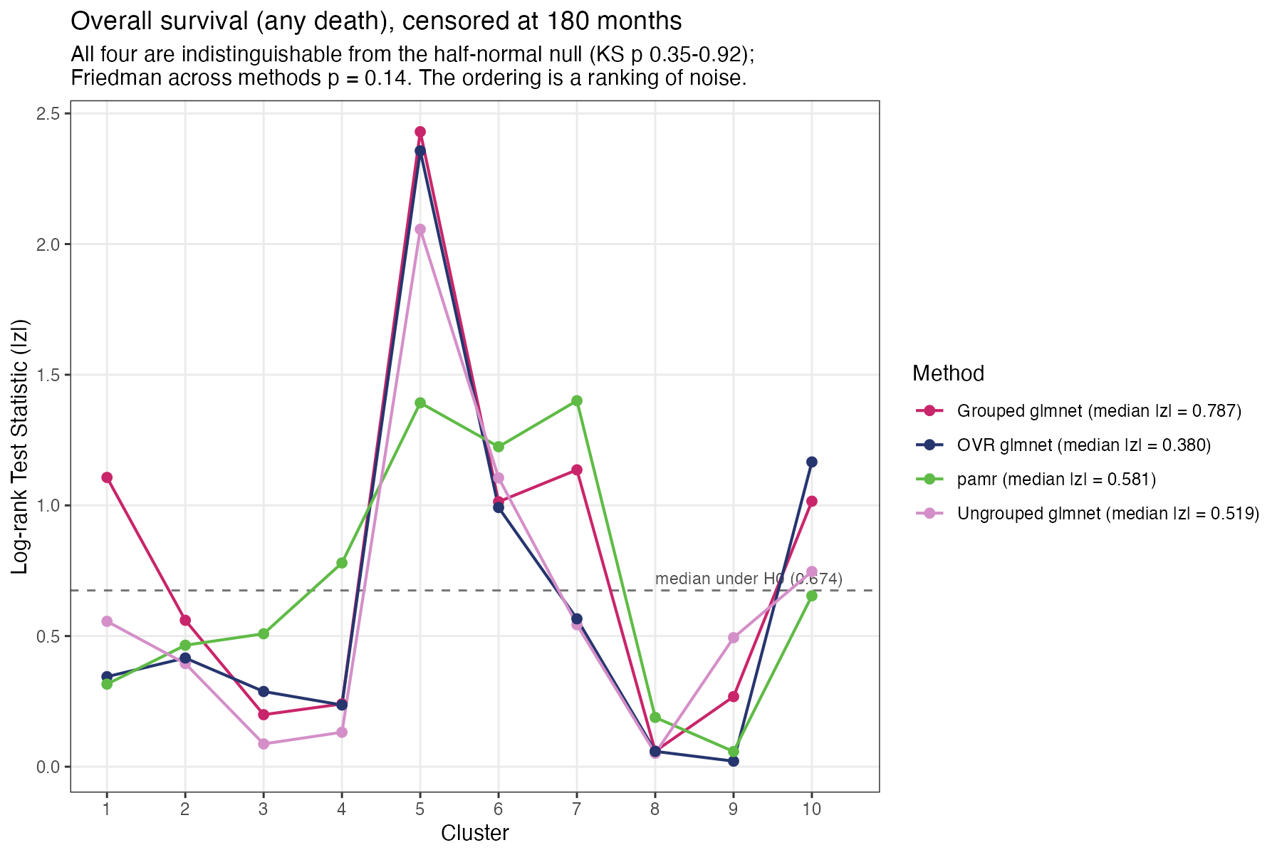
From the data, we compute overall survival, using adminstrative censoring at 180 months per Lazarov and Tibshirani (2026). For each cluster \(k\) and method \(m\) we will compare overall survival using a two-sample long-rank test. The two groups compared are:
- reference — discovery patients whose true label is \(k\)
- comparison — validation patients that \(m\) assigned to \(k\).
For two groups \(z^2 = \chi^2_1\), so \(|z| = \sqrt{\chi^2}\), and small \(|z|\) is read as “this model’s cluster \(k\) survives like the real cluster \(k\)”.
| method | median |z| |
|---|---|
| OVR glmnet | 0.380 |
| Ungrouped glmnet | 0.519 |
| pamr | 0.581 |
| Grouped glmnet | 0.787 |
27.3.1 Kaplan–Meier curves
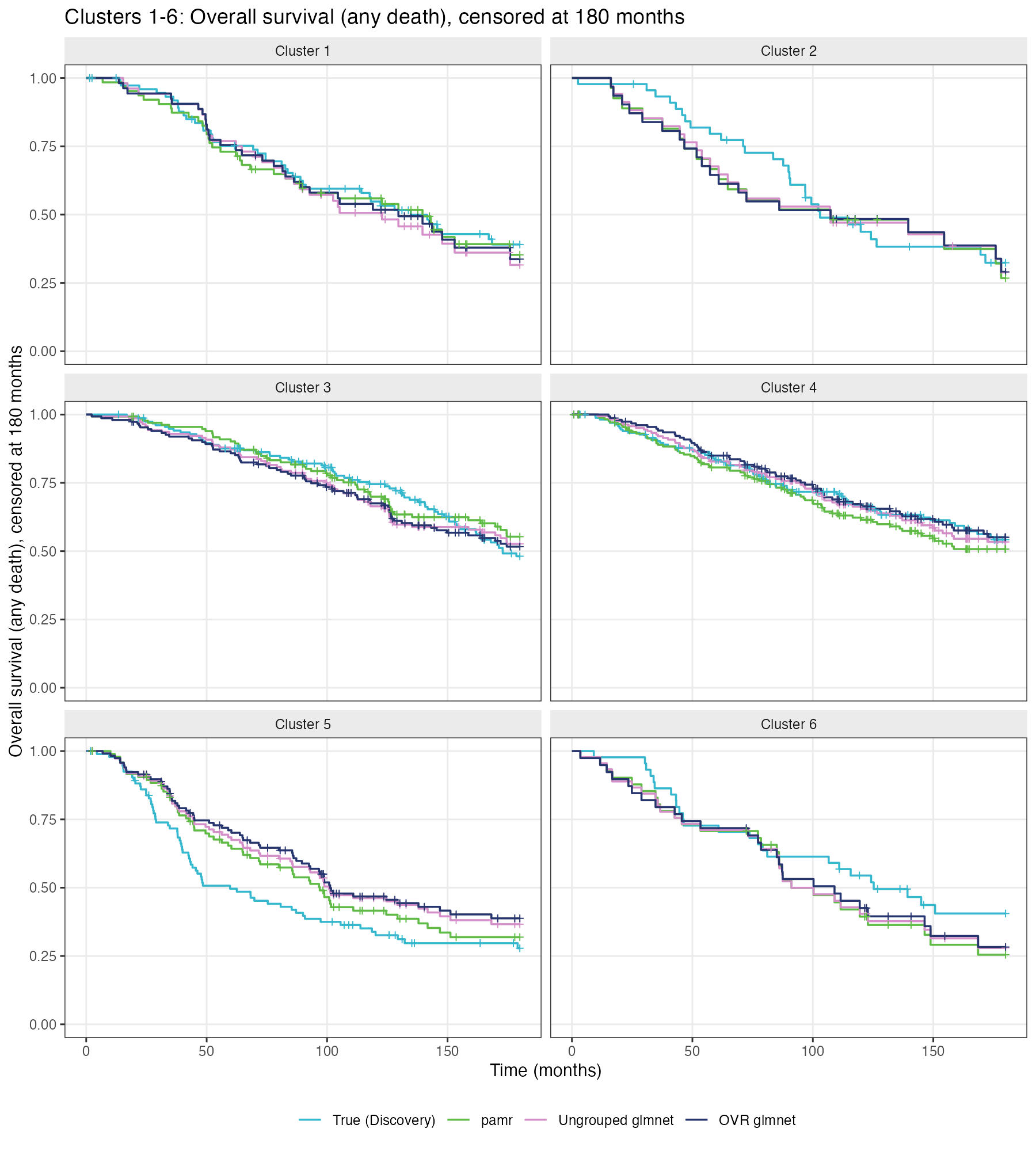
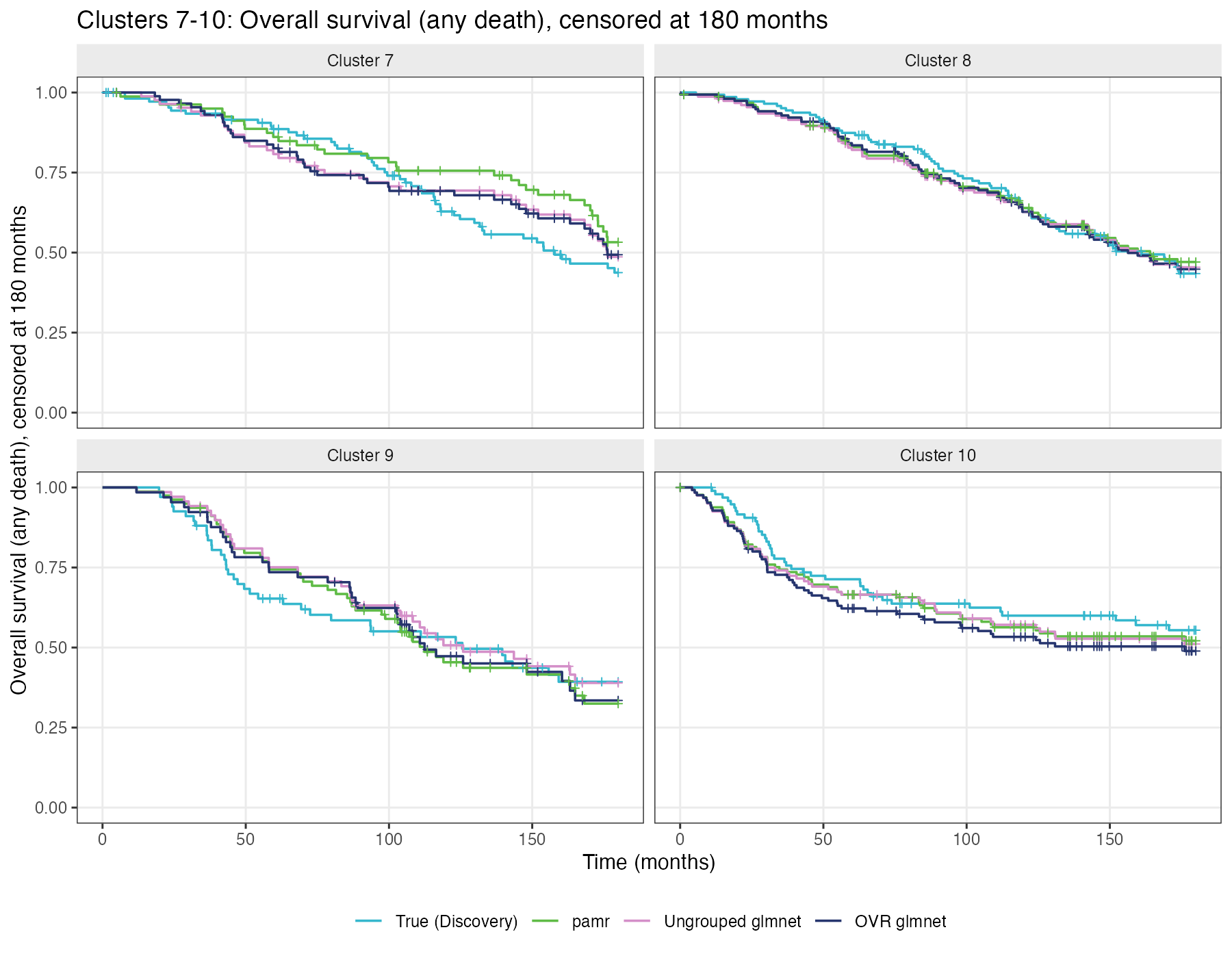
The computed statistic \(|z|\) is asymptotically half-normal and therefore none of the tests would be significant with multiplicities accounted for. Individual comparisons are also small: only 3 of the 40 reach \(|z| > 1.96\), all three of them in cluster 5. Therefore there is nothing to suggest a large difference in survival between the discovery and validation clusters produced by these models.
27.4 Robustness to the fold assignment
In the analysis above, we pre-specified the cross-validation folds. To get some idea of how results can change because of different fold assignments, we can repeat the process with various seeds. Below is a table of results from refitting the same models on the same data across twelve different fold draws:
| quantity | range over 12 draws | analysis results |
|---|---|---|
| Ungrouped union features | 260 – 414 | 267 |
| OVR union features | 401 – 482 | 401 |
| Ungrouped CV error | 0.1234 – 0.1394 | 0.1374 |
pamr CV error |
0.0772 – 0.0883 | 0.0822 |
The CV errors don’t move too much but the selected genes are different. This suggests some robustness in the overall results, but a full-fledged report would detail all the variation in the gene clusters as they could inform biological interpretation.
27.5 Reproducing this chapter results
This case study may be reproduced using the scripts below. See scripts/README.md for details.
scripts/metabric_data.R: assemble and assert the analysis setsscripts/metabric_glmnet.R: fit the four models on shared foldsscripts/metabric_survival.R: perform log-rank analysis on overall survivalscripts/metabric_figures.R: generate remaining figures
The data files are not distributed with this book. Before running the scripts, place the following inputs in data/metabric_raw/:
brca_metabric_clinical_data.tsv: the clinical data export from METABRIC cBioPortalIntClustFeatures_discoverydataset997.txtandIntClustFeatures_validationdataset995.txt: the discovery and validation feature matrices from Supplementary Table S43 of Curtis et al. (2012)