data(MultinomialExample)
x <- MultinomialExample$x
y <- MultinomialExample$y

fit <- glmnet(x, y, family = "multinomial")8 Multiclass classification
In Chapter 7, we considered binary classification problems, where the response variable could take on one of two possible values. In this chapter, we extend our focus to multiclass classification, where the response can take on one of \(K > 2\)$K > 2$ discrete values.
8.1 Multinomial regression model
Assume that the response variable \(G\) takes on values in the set \(\{1,2,\dots, K\}\), where \(K \geq 2\). The linear logistic regression model introduced in Section 7.1 can be generalized to a multi-logit model. There are several ways to do this. Zhu and Hastie (2004) model the probabilities symmetrically: for \(k = 1, \dots, K\), we assume that
\[\text{Pr}(G = k \mid \mathbf{x}) = \dfrac{e^{\beta_{0k} + \mathbf{x}^\top \beta_k}}{\sum_{\ell=1}^K e^{\beta_{0\ell} + \mathbf{x}^\top \beta_\ell}}. \tag{8.1}\]
Here, each class \(k = 1, \dots, K\) gets its own intercept \(\beta_{0k}\) and its own vector of coefficients \(\beta_k = \begin{pmatrix} \beta_{1k} & \dots \beta_{pk} \end{pmatrix}^\top \in \mathbb{R}^p\).1
8.2 Elastic net-regularized multinomial model
The parameterization above is not identifiable without constraints: specifically, for any real value \(c\), the parameters \(\{ \beta_{0k},\beta_k \}_1^K\) and \(\{ \beta_{0k} -c,\beta_k -c \}_1^K\) give identical probabilities in Equation 8.12. However, regularization helps us avoid this ambiguity. For regularized multinomial regression, we follow the approach in Section 7.2 of minimizing the sum of the negative log-likelihood (NLL) and the elastic net penalty. More precisely, the elastic net penalty for this model is
\[\text{Penalty} = \lambda \left[ \frac{1-\alpha}{2} \sum_{j=1}^p \sum_{k=1}^K \beta_{jk}^2 + \alpha \sum_{j=1}^p \sum_{k=1}^K |\beta_{jk}| \right]. \tag{8.2}\]
If we let \(\beta \in \mathbb{R}^{p \times K}\) be the matrix of coefficients where \(\beta_k\) is its \(k\)th column, then Equation 8.2 can be written more succinctly as
\[\text{Penalty} = \lambda \left[ \frac{1-\alpha}{2} \| \beta \|_F^2 + \alpha \sum_{k=1}^K \| \beta_k \|_1 \right],\]
where \(\|\cdot \|_F\) is the Frobenius norm3 and \(\| \cdot \|_1\) is the \(\ell_1\)-norm. The math for the NLL gets a bit tedious and we will spare the reader the details: for more, see Section 4 of Friedman et al. (2010).
8.3 Fitting the model with glmnet
Fitting an elastic net-regularized multinomial model is easy with glmnet(): just include the family = "multinomial" argument:
8.3.1 The predict method
As with family = "binomial" (Section 7.2.1), the predict method for family = "multinomial" can accept
type = "link"(default) to return the linear predictors for each class \(\hat{y}_k = \hat{\beta}_{0k} + \mathbf{x}^\top \hat\beta_k,\;k=1, \dots, K\),type = "response"to return the fitted probabilities for each class \(\hat{p}_k = \dfrac{\exp (\hat{\beta}_{0k} + \mathbf{x}^\top \hat\beta_k)}{1 + \exp (\hat{\beta}_{0k} + \mathbf{x}^\top \hat\beta_k)},\;k=1, \dots, K\), andtype = "class"to return the class label corresponding to the maximum fitted probability.
Here is an example: below, we get the fitted probabilities for each of the first 5 observations of our training data at \(\lambda = 0.1\):
predict(fit, newx = x[1:5, ], s = 0.1, type = "response")
#> , , s=0.1
#>
#>              1         2         3
#> [1,] 0.3079629 0.2816293 0.4104078
#> [2,] 0.2968810 0.4249093 0.2782097
#> [3,] 0.3125643 0.4539161 0.2335196
#> [4,] 0.3198722 0.3676336 0.3124941
#> [5,] 0.3434106 0.4238971 0.2326923
Notice that the each row of the prediction matrix sums to 1, as expected. If we pass type = "class" instead, we get the class label corresponding to the largest entry in each row of the fitted probability matrix:
predict(fit, newx = x[1:5, ], s = 0.1, type = "class")
#>      s=0.1
#> [1,] "3"
#> [2,] "2"
#> [3,] "2"
#> [4,] "2"
#> [5,] "2"
8.3.2 The coef method
The coef method returns the model coefficients at a specific value of the \(\lambda\) tuning parameter. The difference with the models we’ve seen before is the format in which the coefficients are returned. Instead of a single coefficient matrix, coef() returns a list of \(K\) coefficient matrices, with the \(k\)th coefficient matrix corresponding to \(\beta_k\).
model_coefs <- coef(fit, s = 0.1)
length(model_coefs)
#> [1] 3
model_coefs[[2]]  # coefficients for beta_2
#> 31 x 1 sparse Matrix of class "dgCMatrix"
#>                   s=0.1
#> (Intercept)  0.04274176
#> V1           .
#> V2           .
#> V3           .
#> V4           .
#> V5           0.01394588
#> V6           .
#> V7           .
#> V8           .
#> V9          -0.16603691
#> V10          0.14010053
#> V11          .
#> V12          .
....
8.3.3 The plot method
The default plot method gives one coefficient plot for each response:
par(mfrow = c(1, 3))
plot(fit, xvar = "lambda")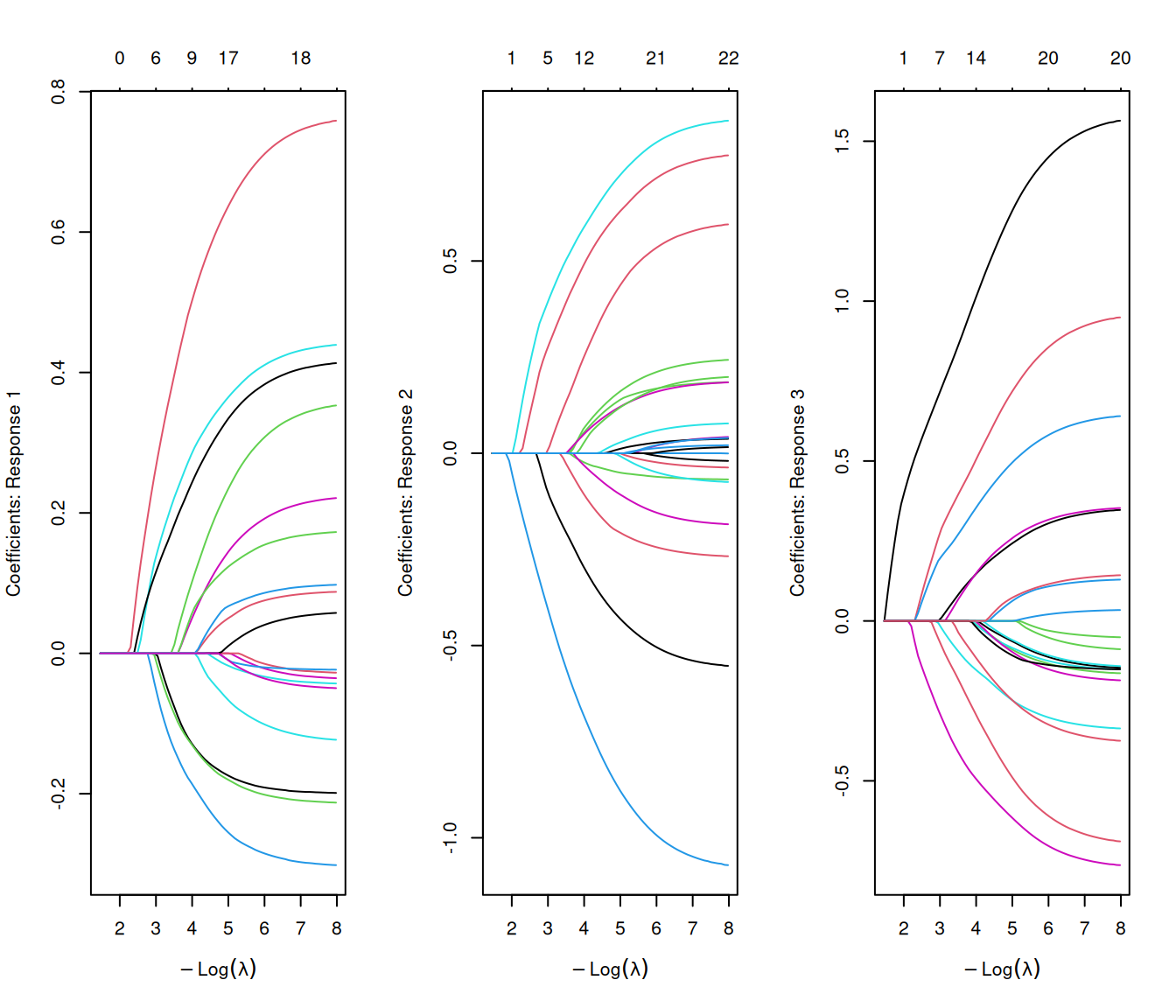
We can set type.coef = "2norm": under this setting, a single curve is plotted per variable, with value equal to the \(\ell_2\) norm of the variable’s coefficient vector.
plot(fit, xvar = "lambda", type.coef = "2norm")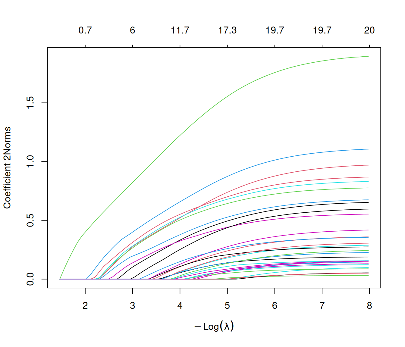
8.3.4 Possibilities for the response
The glmnet function can accept the response variable in the training data in several formats. The example above is probably the most common coding scheme for multinomial data: the response is coded as a numeric vector, with numbers \(1, \dots, K\) representing the \(K\) levels:
str(y)
#>  num [1:500] 3 2 2 2 3 3 3 1 1 1 ...
The response variable can also be passed as a factor.
factor_y <- factor(y, labels = c("A", "B", "C"))
head(factor_y)
#> [1] C B B B C C
#> Levels: A B C
factor_fit <- glmnet(x, factor_y, family = "multinomial")The fit we get is exactly the same, whether the response is passed as a numeric or factor.
If the response is passed as a vector, we can extract the coefficients associated with a particular level with its name:
coef(factor_fit, s = 0.1)[["B"]]
#> 31 x 1 sparse Matrix of class "dgCMatrix"
#>                   s=0.1
#> (Intercept)  0.04274176
#> V1           .
#> V2           .
#> V3           .
#> V4           .
#> V5           0.01394588
#> V6           .
#> V7           .
....
Finally, the response variable can be an nc-column matrix of counts or proportions. Internally glmnet will make the rows of this matrix sum to 1, and absorb the total mass into the weight for that observation.
8.4 A group lasso variation
For the multinomial model, glmnet supports another penalty term besides the elastic net penalty (Equation 8.2). If we let \(b_j\) denote the \(j\)th row of the coefficient matrix \(\beta\)4, we can rewrite the original elastic net penalty as
\[\text{Penalty} = \lambda \left[ \frac{1-\alpha}{2} \| \beta \|_F^2 + \alpha \sum_{j=1}^p \| b_j \|_1 \right]. \tag{8.3}\]
Taking inspiration from the group lasso (Yuan and Lin 2005), we can regularize the NLL with the penalty
\[\text{Penalty} = \lambda \left[ \frac{1-\alpha}{2} \| \beta \|_F^2 + \alpha \sum_{j=1}^p \| b_j \|_2 \right]. \tag{8.4}\]
All that has changed from Equation 8.3 to Equation 8.4 is the \(\ell_1\)-norm in the second term has been replaced with an \(\ell_2\)-norm.
Why do this? The \(\ell_2\) penalty on \(b_j\) has an interesting property: when we fit the model, the elements of \(b_j\) will either be all zero or all non-zero. As a result, an input variable is either included in the model for all levels of the response, or excluded from all levels of the response. This ensures that the same variables are used in the models across the response levels.
To fit this variation, the user just has to pass type.multinomial = "grouped" as an argument to glmnet():
group_fit <- glmnet(x, y, family = "multinomial", type.multinomial = "grouped")The default value is type.multinomial = "ungrouped", which corresponds to Equation 8.2. This default has stayed for historical reasons, but the “grouped” option seems more attractive in terms of providing an interpretable model.
8.5 Additional notes
For algorithmic details on how we solve the minimization problem for the elastic net multinomial model efficiently, see Friedman et al. (2010).
Note that unlike other chapters in this book, in this Chapter \(\beta_k\) refers to a vector of coefficients (those related to level \(k\)) and not a single real number.↩︎
To see this, plug \(\{ \beta_{0k} -c,\beta_k -c \}_1^K\) into Equation 8.1:
\[\frac{e^{\beta_{0k} - c + \mathbf{x}^\top (\beta_k - c)}}{\sum_{\ell=1}^K e^{\beta_{0\ell} - c + \mathbf{x}^\top (\beta_\ell - c)}} = \frac{e^{\beta_{0k} + \mathbf{x}^\top \beta_k} e^{-c(1 + \mathbf{x}^\top \mathbf{1})}}{\sum_{\ell=1}^K e^{\beta_{0\ell} + \mathbf{x}^\top \beta_\ell} e^{-c(1 + \mathbf{x}^\top \mathbf{1})}} = \frac{e^{\beta_{0k} + \mathbf{x}^\top \beta_k}}{\sum_{\ell=1}^K e^{\beta_{0\ell} + \mathbf{x}^\top \beta_\ell}}.\]↩︎
The Frobenius norm of a matrix \(A\) is the square root of the sum of squares of all of its entries: \(\|A\|_F = \sqrt{ \sum_{i=1}^m \sum_{j=1}^n A_{ij}^2 }\) .↩︎
For avoidance of doubt: In this chapter, \(\beta\) is a \(p \times K\) matrix of coefficients, \(\beta_k\) refers to its \(k\)th column, and \(b_j\) refers to its \(j\)th row.↩︎