data(PoissonExample)
x <- PoissonExample$x
y <- PoissonExample$y

fit <- glmnet(x, y, family = "poisson")9 Poisson regression
9.1 The Poisson regression model
Poisson regression is often used to model a response variable when it is a count. There are many examples of count responses across many domains, here are some examples:
Ecology: Species count, number of sightings of a particular species
Epidemiology: Disease incidence (number of new cases of a disease)
Incident response: Number of emergency calls, number of incidents of a particular type (e.g. fire, medical)
Sports: Player statistics (e.g. number of goals, points, assists)
Sales: Number of purchases
Poisson regression is suited for modeling counts as it assumes that the response can only take on non-negative integer values \(\{ 0, 1, 2, \dots \}\), whereas ordinary least squares (OLS) allows response predictions to be fractional or even negative.
Let \(y\) denote the response variable, which can only take on non-negative integer values \(\{ 0, 1, 2, \dots \}\). We can model \(y\) as follows:
\[y \sim \text{Poi}(\mu(\mathbf{x})), \qquad \log \mu(\mathbf{x}) = \eta(\mathbf{x}) = \beta_0 + \beta^\top \mathbf{x}, \tag{9.1}\]
where \(\text{Poi}(\mu)\) is a Poisson distribution with mean \(\mu > 0\).1
As with logistic regression (Chapter 7), we can estimate \(\beta_0\) and \(\beta\) from a training dataset by minimizing the negative log-likelihood (NLL) of the data. In the Poisson model, for observation \(i\), the implied mean for response \(y_i\) is \(\mu_i = \exp (\beta_0 + \beta^\top \mathbf{x}_i)\). The log-likelihood for observation \(i\) is
\[\begin{aligned} \ell(y_i, \mu_i) &= \log \left[ \frac{\mu_i^{y_i} e^{-\mu_i}}{y_i !} \right] \\ &= y_i \log \mu_i - \mu_i - \log (y_i !). \end{aligned}\]
The Poisson regression coefficient vector is obtained by solving
\[\begin{aligned} (\hat\beta_0, \hat\beta) &= \underset{(\beta_0, \beta) \in \mathbb{R}^{p+1}}{\text{argmin}} \; -\sum_{i=1}^n \ell (y_i, \beta_0 + \mathbf{x}_i^\top \beta) \\ &= \underset{(\beta_0, \beta) \in \mathbb{R}^{p+1}}{\text{argmin}} \; -\sum_{i=1}^n \left[ y_i (\beta_0 + \beta^\top \mathbf{x}_i) - e^{\beta_0 + \beta^\top \mathbf{x}_i} \right]. \end{aligned}\]
We can fit the Poisson regression model in R with the glm function from the stats package, specifying the option family = poisson.
9.2 Regularized Poisson regression
To extend the lasso and elastic net models to the count-response setting, we follow the same strategy as in Section 7.2: instead of minimizing just the NLL, we minimize a weighted sum of the NLL and the elastic net penalty:
\[(\hat\beta_0, \hat\beta) = \underset{(\beta_0, \beta) \in \mathbb{R}^{p+1}}{\text{argmin}} \; -\frac{1}{n} \sum_{i=1}^n \ell (y_i, \beta_0 + \mathbf{x}_i^\top \beta) + \lambda \left(\frac{1-\alpha}{2}\|\beta \|_2^2 + \alpha \|\beta \|_1 \right).\]
We can fit elastic net-regularized Poisson regression models with glmnet() by passing the family = "poisson" argument:
9.2.1 The predict method
For family = "poisson", the default value returned by the predict method is the linear predictor \(\hat\eta(\mathbf{x})=\log (\hat{\mu}(\mathbf{x})) = \hat{\beta}_0 + \mathbf{x}^\top \hat\beta\). To get the mean estimates \(\hat{\mu}(\mathbf{x}) = \exp (\hat{\beta}_0 + \mathbf{x}^\top \hat\beta)\) directly, pass type = "response" .
We see evidence of this in the plot below. When we plot the return values of predict() with type = "response" against the default predict() values, all the points lie on the curve \(y = \exp(x)\).
lin_pred <- predict(fit, newx = x[1:10,], s = 0.01)
mean_pred <- predict(fit, newx = x[1:10,], type = "response", s = 0.01)
plot(lin_pred, mean_pred, pch = 16)

x_grid <- seq(from = min(lin_pred), to = max(lin_pred), length.out = 101)
lines(x_grid, exp(x_grid), col = "red")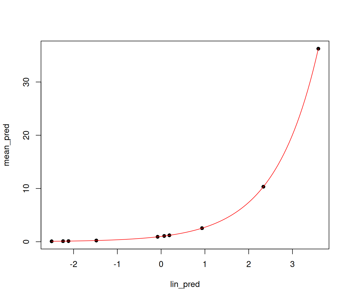
9.3 Accounting for different exposure lengths
When dealing with rate data in Poisson models, the counts collected are often based on different exposures such as length of time observed, area and years. When using the training data, the model needs to account for differing exposures across observations.
To fix ideas, suppose we are counting beetles at a particular location for a certain amount of time. Assume that for observation 1, we went to location 1, measured input variables \(\mathbf{x}_1\) characterizing this location, and counted the number of beetles \(y_1\) seen in 1 minute. For observation 2, we went to a similar location having the same input variable values \(\mathbf{x}_2 = \mathbf{x}_1\), but we counted the number of beetles \(y_2\) seen in 30 minutes. It would not make sense for the model to estimate the fitted means for \(y_1\) and \(y_2\) to be the same: \(\exp(\beta_0 + \beta^\top \mathbf{x}_1) = \exp(\beta_0 + \beta^\top \mathbf{x}_2)\). We run into this issue because we did not account for differing length of exposure across the two observations.
A better way to model such data would be to model the rate \(\mu(\mathbf{x})\) relative to a unit exposure time. If an observation \(y_i\) was exposed for \(E_i\) units of time, then the expected count (mean) would be \(\mu_i = E_i \mu(\mathbf{x}_i)\), and the log-mean would be \(\log \mu_i = \log E_i + \log \mu(\mathbf{x}_i)\). For the example in the previous paragraph, if a minute is the unit of exposure time, then \(E_1 = 1\), \(E_2 = 30\), we would estimate the same unit rate \(\mu(\mathbf{x}_2) = \mu(\mathbf{x}_1)\) but different fitted means \(\mu_1 = \mu(\mathbf{x}_1)\) and \(\mu_2 = 30 \mu(\mathbf{x}_2)\).
Here amount of measurement time represents exposure. It could be size of the region sampled, or many similar variations.
How does this affect our Poisson regression model? For each observation \(i\), on top of input and output variables \((\mathbf{x}_i, y_i)\) we need to collect exposure lengths \(E_i\). The Poisson regression model (Equation 9.1) becomes
\[y_i \sim \text{Poi}(\mu_i), \qquad \log \mu_i = \log E_i + \beta_0 + \beta^\top \mathbf{x}_i,\]
Notice that the structural form of the model is the same! The only difference is that in the model for \(\mu_i\), the intercept term \(\beta_0\) is replaced by \(\log E_i + \beta_0\). We call \(\log E_i\) the offset.
9.3.1 Model offsets in glmnet
glmnet allows the user to pass in a vector of length equal to the number of observations as an offset via the offset argument. In the context of Poisson regression, you should pass the \(\log E_i\) values as the offset vector. Here is an artificial example:
set.seed(1)
exposure <- sample(1:10, size = length(y), replace = TRUE)

fit <- glmnet(x, y, family = "poisson", offset = log(exposure))
The returned fit object behaves as it would if we didn’t pass the offset argument to glmnet. The only difference happens when we try to make predictions. If offsets are supplied to glmnet() during training time, we need to give offsets to predict as well via the newoffset option to get predictions, if not we get an error:
predict(fit, newx = x[1:5,], s = 0.01)
#> Error:
#> ! No newoffset provided for prediction, yet offset used in fit of glmnetpredict(fit, newx = x[1:5,], s = 0.01, newoffset = log(exposure[1:5]))
#> s=0.01
#> [1,] 1.4347742
#> [2,] 1.8868950
#> [3,] -2.9004806
#> [4,] -1.7920835
#> [5,] -0.9458622One way to tell if offsets were used in training the model is to inspect the offset element of the object returned by glmnet: it is TRUE if offsets were used, and FALSE otherwise.
fit$offset
#> [1] TRUE
Caution
For Poisson regression, the offset vector should be the log of the exposures, \(\log E_i\), not the exposures themselves.
Like the Gaussian and binomial models, the Poisson distribution is a member of the exponential family of distributions, which is a reason for its widespread use.↩︎