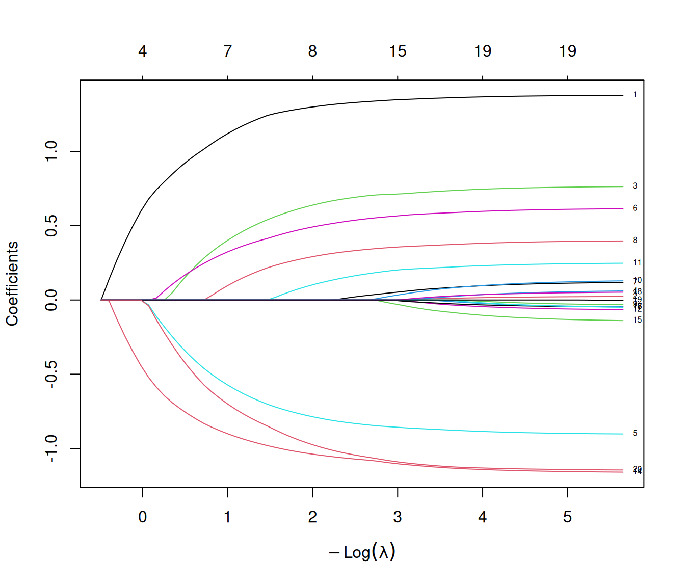
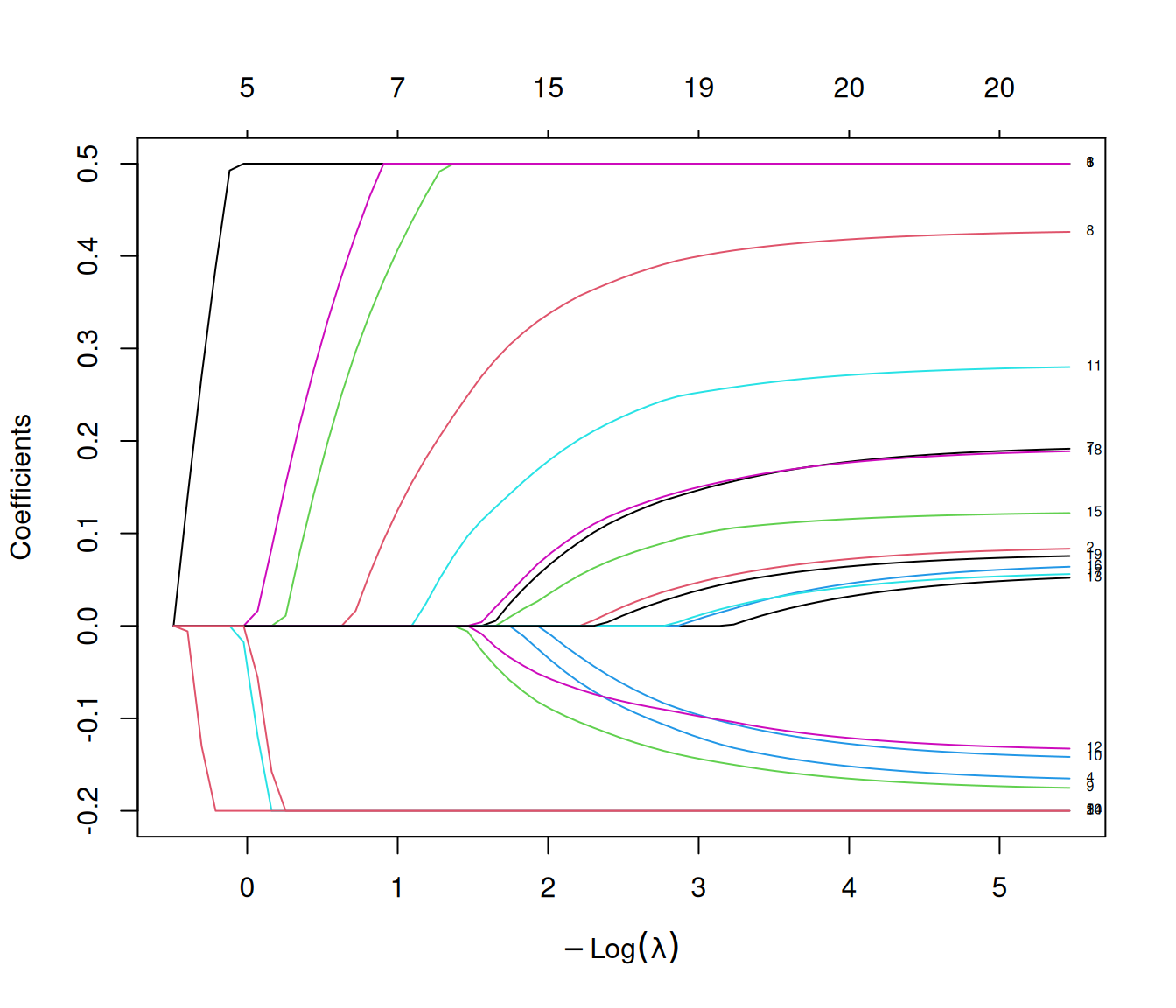
Suppose we want to fit our model but limit the size of the coefficients. If we want the coefficients to be no larger than \(U\) and/or no smaller than \(L\), we can specify upper.limits = U and/or lower.limits = L In the glmnet call. Here is an example:
data("QuickStartExample")x <- QuickStartExample$xy <- QuickStartExample$y# original coefficient plotoriginal_fit <-glmnet(x, y)plot(original_fit, xvar ="lambda", label =TRUE)# coefficient plot with limitsbound_fit <-glmnet(x, y, upper.limits =0.5, lower.limits =-0.2)plot(bound_fit, xvar ="lambda", label =TRUE)
Note
The upper.limits and lower.limits constraints on the coefficients are always on the original scale of the features, regardless of whether the standardize option is set to TRUE or FALSE.
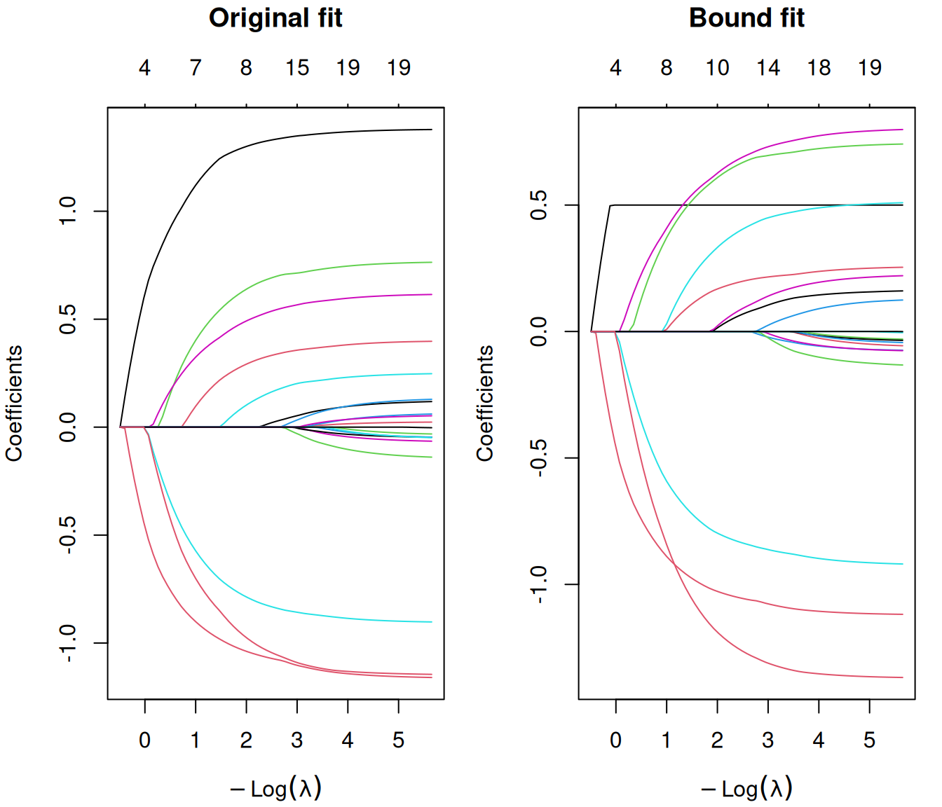
It is possible for the coefficient limits to vary for each factor: simply pass a vector to the upper.limits and/or lower.limits argument. (If a scalar is passed, as in the example above, the same limit is used across all features.) You can keep some feature coefficients unbounded in the positive or negative direction: set the corresponding element of upper.limits or lower.limits to Inf or -Inf respectively.
Here is an example where we only put an upper bound on feature 1. Notice that the coefficients for the other features change as well: the coefficients for other features have to adjust to compensate for the additional constraint on feature 1.
upper_limits <-c(0.5, rep(Inf, ncol(x) -1))bound_fit <-glmnet(x, y, upper.limits = upper_limits)# original coefficient plot vs. bound plotpar(mfrow =c(1, 2), mar =c(4,4,4,1))plot(original_fit, xvar ="lambda", label =TRUE); title("Original fit", line =3)plot(bound_fit, xvar ="lambda", label =TRUE); title("Bound fit", line =3)
16.1 The non-negative lasso
An important use case of these function arguments is when we want all the coefficients to be non-negative: this is known as the non-negative lasso. To achieve this, we can simply set lower.limits = 0.
One use case of the non-negative lasso is index tracking in finance (Wu et al. 2014). Assume that the response variable \(y\) is the return of an index and our input features \(x_1, \dots, x_p\) are the returns of \(p\) stocks. We want to construct a portfolio of these stocks such that the portfolio return closely tracks the return of the index. In such an application, we might want to restrict the coefficients (representing how much of each stock we are buying) to be non-negative to ensure a long-only portfolio.
16.2 The Unilasso
The uniLasso(Chatterjee et al. 2025) is a version of lasso that is heavily influenced by the univariate fits of each feature. Features with strong univariate fits get favored, and in addition the the final lasso fit is constrained to respect the signs of the inivariate fits. The idea is to get a sparser and more interpretable model, without much loss (if any) in accuracy. There is an R package uniLasso on CRAN that implements these models. Here we present a particular version using penalty weights and coefficient bounds. The idea is to:
Compute the univariate coefficients for each feature, and use them to construct penalty factors for the adaptive lasso.
In addition, constrain the signs of the lasso coefficients to be the same as the sign of the univariate coefficients.
We demonstrate using our simple example. We first compute the univariate coefficients for each of the features, and use them to construct a penalty factor for the adaptive lasso.
xs =scale(x, TRUE, FALSE) # center each of the columnsnxs =colSums(xs^2) # sum of squares of each centered featureubeta =t(xs) %*% y / nxs # univariate LS coefficientspf =1/abs(ubeta)
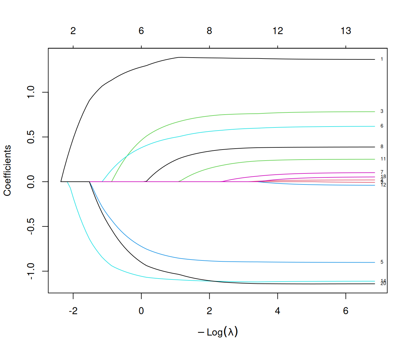
Next we fit a lasso using this penalty factor, but also restrict the signs of the coefficients to match those of the univariate fit.
We see the fit is sparser than the earlier lasso fit. We would have to perform cross-validation to select lambda with care. In each training fold, we would want to redo the univariate fits and recompute the penalty factor each time. The uniLasso package avoids this extra layer at the second stage by using LOO univariate regressions (leave-one-out) at the first stage; see the paper and package for more details.
Chatterjee, Sourav, Trevor Hastie, and Robert Tibshirani. 2025. “Univariate-GuidedSparseRegression.”Harvard Data Science Review 7 (3).
Wu, Lan, Yuehan Yang, and Hanzhong Liu. 2014. “Nonnegative-Lasso and Application in Index Tracking.”Computational Statistics & Data Analysis 70 (February): 116–26. https://doi.org/10.1016/j.csda.2013.08.012.