3  Details on the lambda sequence

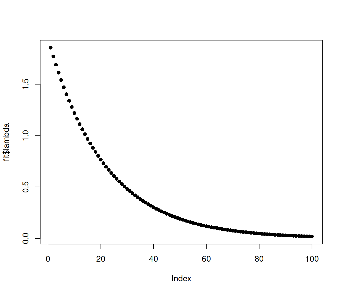
The coefficients of the elastic net are given by

\[\min_{\beta_0, \mathbf{\beta}} \quad \frac{1}{2n} \| \mathbf{y} - \beta_0 \mathbf{1} - \mathbf{X\beta} \|_2^2 + \lambda \left(\frac{1-\alpha}{2}\|\beta \|_2^2 + \alpha \|\beta \|_1 \right),\] where \(n\) is the number of observations in the dataset and \(\lambda \geq 0\) and \(\alpha \in [0,1]\) are hyperparameters chosen by the user. As mentioned in Section 2.6, we recommend choosing \(\alpha\) based on the type of prediction model you want. Assume that you’ve fixed the value of \(\alpha\). How can you choose the value of \(\lambda\) for your application?

3.1 Some general intuition

In general, larger values of \(\lambda\) lead to sparser models. One possibility for your application is to pick a value of \(\lambda\) that meets your sparsity needs. For example, you could set \(\lambda\) corresponding to the most expressive model (in terms of deviance explained) with no more than \(K\) non-zero coefficients, where \(K\) is chosen based on other business objectives or constraints.

3.2 The lambda path

It is difficult a priori to know which value of \(\lambda\) works best for a given application. Because of this, glmnet fits the elastic net model for a path of \(\lambda\) values \(\lambda_1 > \lambda_2 > \dots\), and not for a single value of \(\lambda\). This gives the user a range of models to choose from. In particular, we start the path at \(\lambda_1\) large enough so that the corresponding elastic net model is the sparsest possible model: \(\hat\beta(\lambda_1) = \mathbf{0}\).

We note that the computational cost of fitting the elastic net model for several \(\lambda\) values does not scale linearly with the number of \(\lambda\) values, i.e. it is not the case that fitting the model for a path of 100 \(\lambda\) values takes 100 times as long as fitting the model for a single \(\lambda\) value. There are few reasons for this:

• If \(\lambda_1 > \lambda_2\) are not too different, then the elastic net solutions corresponding to \(\lambda_1\) and \(\lambda_2\), denoted by \(\hat\beta(\lambda_1)\) and \(\hat\beta(\lambda_2)\), are not too different as well. When solving for \(\hat\beta(\lambda_2)\), warm-starting the algorithm at \(\hat\beta(\lambda_1)\) enables it to converge to \(\hat\beta(\lambda_2)\) quickly.

• In coordinate descent, the algorithm typically has to loop through all \(p\) elements of the coefficient vector \(\beta\). Recall that \(p\) is the number of features in our dataset, which is usually large in applications for the elastic net. However, by using heuristics known as strong rules (Tibshirani et al. 2011), we can predict accurately which features will have coefficient zero; we can exclude these coefficients from the coordinate descent loop.

3.2.1 Arguments for the lambda path

You can specify the lambda path explicitly by passing a vector of lambda values to the lambda argument. However, we generally recommend that users leave this argument blank and let glmnet compute its own lambda sequence based on nlambda and lambda.min.ratio (discussed below). This is because (i) the user typically does not know a priori which lambda value to use, and (ii) glmnet ’s implementation uses warm starts for speed and so fits an entire path of models very efficiently.

When lambda is left blank, glmnet computes \(\lambda_{max}\), the smallest value of \(\lambda\) such that the estimated coefficients would be all equal to zero¹. The program then computes \(\lambda_{min}\) such that the ratio \(\lambda_{min} / \lambda_{max}\) is equal to lambda.min.ratio. (lambda.min.ratio defaults to \(10^{-2}\) if the number of variables exceeds the number of observations, and defaults to \(10^{−4}\) otherwise). The lambda sequence which glmnet fits models for has nlambda values (default 100), starting at \(\lambda_{max}\) and ending at \(\lambda_{min}\). The lambda values are equally spaced on the log scale.

set.seed(1)
n <- 50; p <- 100
x <- matrix(rnorm(n * p), nrow = n)
y <- rowSums(x[, 1:10]) + rnorm(n)

fit <- glmnet(x, y)

# default lambda sequence
plot(fit$lambda, pch = 16)

# default lambda sequence on log scale (relative to lambda_max)
plot(log10(fit$lambda) - log10(fit$lambda)[1], pch = 16)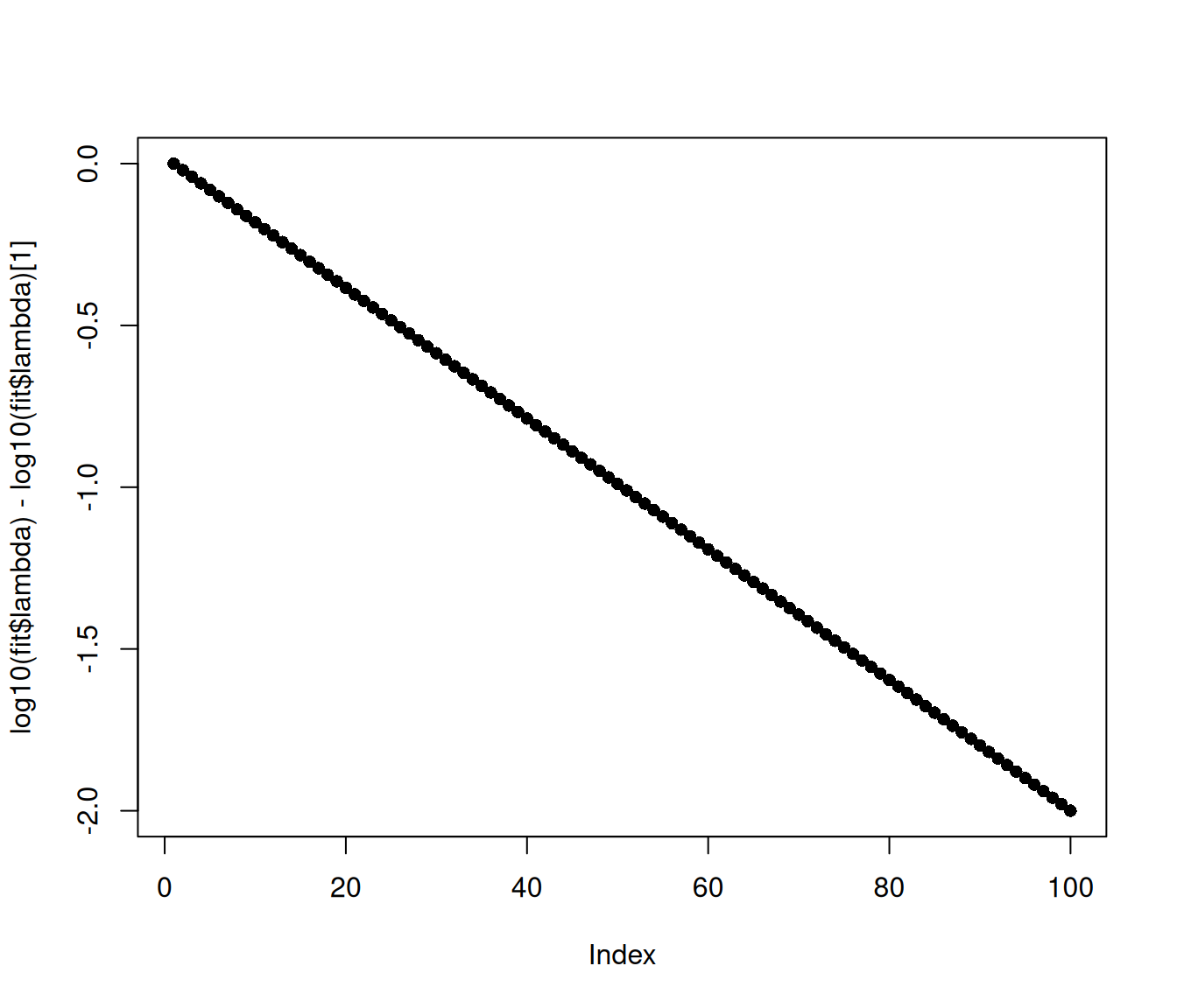

Here is an example of fitting elastic net models with user-defined nlambda and lambda.min.ratio:

# different nlambda and lambda.min.ratio values
fit <- glmnet(x, y, nlambda = 10, lambda.min.ratio = 1E-1)
plot(log10(fit$lambda) - log10(fit$lambda)[1], pch = 16)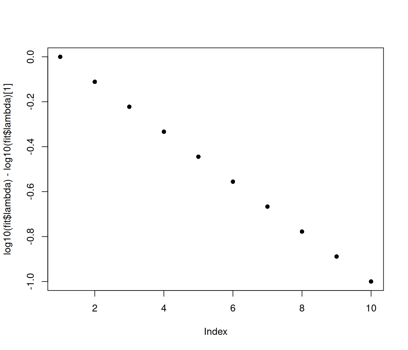

3.2.2 Early stopping

While the arguments above help us explicitly define the \(\lambda\) values at which glmnet will fit the model, we would like to terminate the algorithm early if, at some point, our model explains almost all of the variability in the observations.

To this end, we define the deviance of a model with parameter \(\beta\) to be

\[D(\beta) = 2(\ell_{saturated} - \ell(\beta)),\]

where \(\ell_{saturated}\) is the maximum log-partial likelihood when the predicted responses may vary freely, and \(\ell(\beta)\) is the log-partial likelihood when we use the model. Similarly, we define the null deviance to be

\[D_{null} = D(0) = 2(\ell_{saturated} - \ell_{null}),\] where \(\ell_{null} = \ell(0)\). At a given step, we terminate the algorithm early if more than 99.9% of the null deviance is explained by the model, i.e. if

\[D^2= 1-D(\beta_{current}) / D_{null} \geq 0.999.\]

This measure, the percent deviance explained, generalizes the common \(R^2\) statistic (percent of null variance)explained

3.3 What is an optimal value of \(\lambda\)?

One general approach to choosing \(\lambda\) is to use out-of-sample prediction error to guide this choice.

If your application has an abundance of observations, you can split your data into two sets: a training set and a validation set. (A 70-30 split between the training and validation sets is a good rule of thumb.) Fit your model for the entire range of \(\lambda\) values on the training set, compute the prediction error on the validation set, then pick the value of \(\lambda\) that gives the best prediction error.

If you cannot afford (data wise) to split your data into training and validation sets, our recommended approach is cross-validation, which is the subject of our next chapter.

Tibshirani, Robert, Jacob Bien, Jerome Friedman, et al. 2011. “Strong Rules for Discarding Predictors in Lasso-Type Problems.” Journal of the Royal Statistical Society Series B: Statistical Methodology 74 (2): 245–66. https://doi.org/10.1111/j.1467-9868.2011.01004.x.

---

1. When \(\alpha=0\), \(\lambda_{max}\) is infinite, i.e. some coefficient will always be non-zero for finite \(\lambda\). To avoid such extreme values of \(\lambda_{max}\), if \(\alpha < 0.001\) we return the \(\lambda_{max}\) value for \(\alpha=0.001\).