data("QuickStartExample")
x <- QuickStartExample$x
y <- QuickStartExample$y

penalty_factor <- rep(1, ncol(x))
penalty_factor[c(1, 3)] <- 0
pfit <- glmnet(x, y, penalty.factor = penalty_factor)
plot(pfit, label = TRUE)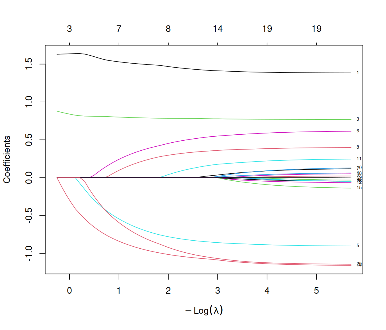
The coefficients of the elastic net are given by
\[\min_{\beta_0, \mathbf{\beta}} \quad \frac{1}{2n} \| \mathbf{y} - \beta_0 \mathbf{1} - \mathbf{X\beta} \|_2^2 + \lambda \left(\frac{1-\alpha}{2}\|\beta \|_2^2 + \alpha \|\beta \|_1 \right).\]
Let’s write the penalty term a bit more explicitly:
\[\begin{aligned} \lambda \left(\frac{1-\alpha}{2}\|\beta \|_2^2 + \alpha \|\beta \|_1 \right) &= \lambda\sum_{j=1}^p \left( \frac{1 - \alpha}{2} \beta_j^2 + \alpha |\beta_j| \right). \end{aligned}\]
For each feature \(j\), the elastic net penalty is a combination of its squared value and absolute value, multiplied by a global parameter \(\lambda\).
A simple generalization of the elastic net penalty is to allow different penalties \(\lambda_j\) for each of the variables. We implement this via penalty scaling parameters \(\gamma_j \geq 0\). If \(\gamma_j > 0\), then the penalty applied to \(\beta_j\) is \(\lambda_j = \lambda \gamma_j\):
\[\min_{\beta_0, \mathbf{\beta}} \quad \frac{1}{2n} \| \mathbf{y} - \beta_0 \mathbf{1} - \mathbf{X\beta} \|_2^2 + \lambda \sum_{j=1}^p \gamma_j \left( \frac{1 - \alpha}{2} \beta_j^2 + \alpha |\beta_j| \right). \tag{19.1}\]
The default is \(\gamma_j = 1\) for all \(j\), i.e. coefficients are penalized equally.
We can specify penalty factors in glmnet via the penalty.factor argument. penalty.factor is always internally rescaled to sum to nvars, the number of variables in the given x matrix, before being used for fitting.
Here we have illustrated penalty factors for the Gaussian models, but of course the same idea applies to all the models fit by glmnet.
Variable penalty factors can be used to incorporate prior knowledge in our model. If we believe that some variables are more important than others for predicting the response, we can give these variables a smaller penalty factor. This will encourage these variables to stay in the model. Here are some possible use cases:
If you have feature importance scores from another model (e.g. importance scores from a random forest model), you can set the penalty factors to be inversely proportional to these scores so that more important features are penalized less.
In a medical application, prior clinical work might indicate that some biomarkers are crucial to predicting the outcome. We would want to decrease the penalty factor on these features so that they are encouraged to stay in the model.
An important special case of the penalty factor is when \(\gamma_j = 0\) for one or more features. If \(\gamma_j = 0\), variable \(j\) does not get penalized, and always enters the model unrestricted at the first step and remains in the model. This is useful in the case where some variables are always to be included unpenalized in the model, such as a treatment indicator variable or demographic variables like sex and age in medical studies.
Here is an example where we set the penalty factor for features 1 and 3 to be zero. We can see from the coefficient plot that these two features always stay in the model, i.e. have non-zero coefficients.
data("QuickStartExample")
x <- QuickStartExample$x
y <- QuickStartExample$y
penalty_factor <- rep(1, ncol(x))
penalty_factor[c(1, 3)] <- 0
pfit <- glmnet(x, y, penalty.factor = penalty_factor)
plot(pfit, label = TRUE)
Penalty rescaling can be used to implement the adaptive lasso (Zou 2006). The adaptive lasso was proposed as a variant of the lasso that has certain “oracle” properties. Loosely speaking, it means that the adaptive lasso correctly identifies the subset of features which are in the true model, and it estimates the coefficient values at the optimal rate. (See Section 19.5 for a technical description of these properties.)
The adaptive lasso algorithm is easy to describe. Assume that the input and response variables are mean-centered so that we can ignore the intercept term. First, obtain some (rough) estimate of the coefficient vector \(\hat\beta\): common choices include coefficients from ordinary least squares (OLS) or ridge regression1. Next, pick \(\gamma > 0\), and define weights \(\hat{w}_j = 1 / |\hat\beta |^\gamma\) for \(j = 1, \dots, p\). Finally, the adaptive lasso coefficient estimates are given by the minimization problem
\[\hat\beta^* = \underset{\beta}{\text{argmin}} \; \frac{1}{2n} \left\|\mathbf{y} - \mathbf{X}\beta \right\|_2^2 + \lambda \sum_{j=1}^p \hat{w}_j |\beta_j|. \tag{19.2}\]
Equation 19.2 is exactly Equation 19.1, and thus can be solved directly with glmnet() with the correct penalty factors. (The \(\gamma\) hyperparameter can be chosen via cross-validation; a common choice in practice is \(\gamma = 1\).)
Here is an implementation of the adaptive lasso with the first stage estimate being ridge regression coefficients:
# need to remove the intercept term from the coefficients
set.seed(1)
ridge_fit <- cv.glmnet(x, y, alpha = 0)
ridge_coefficients <- coef(ridge_fit, s = "lambda.min")
ridge_coefficients <- ridge_coefficients[2:length(ridge_coefficients)]

# get penalty factors and fit adaptive lasso
gamma <- 1
pen_factors <- 1 / abs(ridge_coefficients)^gamma
adaptive_lasso_fit <- glmnet(x, y, penalty.factor = pen_factors)
If we were to do cross-validation, we would have to include the ridge fit in each fold to avoid severe bias from data snooping! The next section shows how we can do that seamlessly.
Similar to the dynamic exclude argument in Chapter 18, the penalty.factor argument can be a function. We illustrate this using a simplified version of the adaptive lasso above where the penalty factor depends on the univariate regression coefficients. Like there, the penalty factor will be inversely proportional to the size of these coefficients.
We write a simple function to compute these coefficients and the penalty factors.
pf <- function(x, y, ...){
  x <- scale(x, TRUE, FALSE) # remove the column means
  beta <- t(y) %*% x / colSums(x^2) # univariate coefficients
  1/abs(beta)
}
Now we pass this function in as the penalty factor for cv.glmnet on our simple example. This means the penalty factors get computed separately in each training fold, so that leakage is avoided. Although we do not expect to see much on this simple example, it does deliver a slightly smaller model with lower CV error.
par(mfrow=c(2,1))
set.seed(1)
fitcv <- cv.glmnet(x,y, penalty.factor = pf)
plot(fitcv)
print(fitcv)
#>
#> Call:  cv.glmnet(x = x, y = y, penalty.factor = pf)
#>
#> Measure: Mean-Squared Error
#>
#>     Lambda Index Measure     SE Nonzero
#> min 0.1613    46   1.024 0.1105       8
#> 1se 0.6511    31   1.127 0.1661       7
mtext("Adaptive Lasso",3,2.3)
set.seed(1)
fitcv0 <- cv.glmnet(x,y)
plot(fitcv0)
mtext("Lasso",3,2.3)
print(fitcv0)
#>
#> Call:  cv.glmnet(x = x, y = y)
#>
#> Measure: Mean-Squared Error
#>
#>      Lambda Index Measure     SE Nonzero
#> min 0.08307    33   1.075 0.1251       9
#> 1se 0.15933    26   1.175 0.1374       8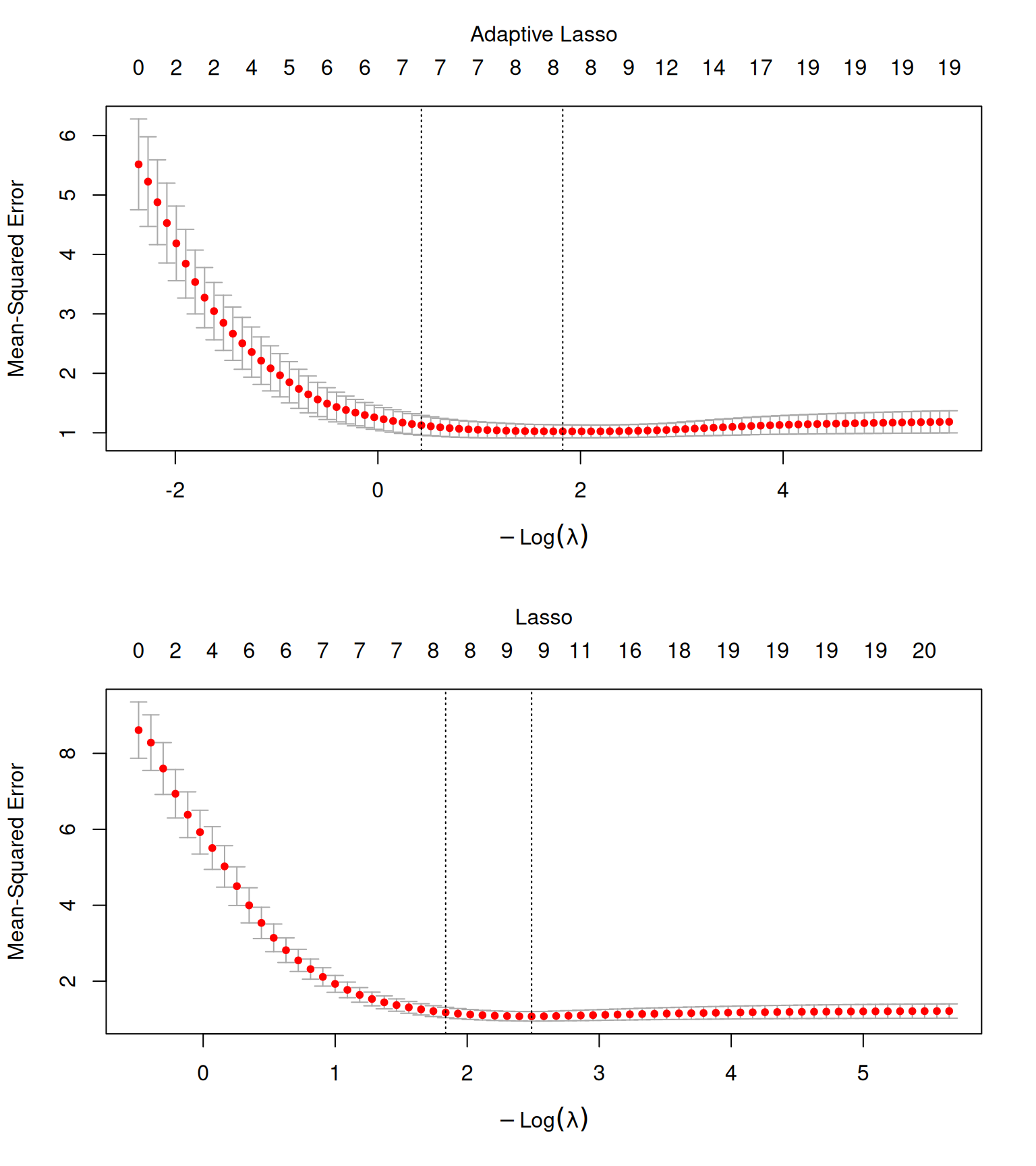
As in Section 18.4, we can allow for additional arguments to the penalty function by embedding it within a generator function that has as input these additional arguments.
Assume that the response \(y\) is related to the input features\(\mathbf{x} = \begin{pmatrix} x_1 & \dots & x_p \end{pmatrix}\) according to
\[\mathbb{E}[y \mid \mathbf{x}] = \beta_1^* x_1 + \dots + \beta_p^* x_p.\]
Let \(\mathcal{A} = \{ j: \beta_j^* \neq 0\}\) denote the subset of predictors which the response \(y\) depends on, and assume that \(|\mathcal{A}| = p_0 < p\). Let \(\hat{\beta}(\delta)\) denote the coefficient vector produced by the procedure \(\delta\). \(\delta\) is said to be an oracle procedure if \(\hat\beta(\delta)\) asymptotically has the following properties:
Zou (2006) show that the adaptive lasso enjoys these oracle properties.
Actually we don’t have to use the OLS estimate for the coefficients: any \(\sqrt{n}\)-consistent estimator to \(\beta^*\) will do.↩︎